On the generation of direction numbers for Sobol sequences and their application to Quasi Monte Carlo methods
Monte Carlo (MC) methods lie at the heart of many numeric computing tasks ranging from modelling how high velocity ions impinging on an atomic lattice to the pricing of a financial instruments. While being generic and scaling independently of problem dimension, practical applications of Monte-Carlo suffers from the slow error convergence rate of as the number of simulations, , increases. Thus, achieving high precision estimates with Monte Carlo often requires large numbers of simulations. Quasi-Monte Carlo methods attempt to accelerate this by replacing the pseudo-random sequences in MC with deterministic `low discrepancy` sequences that have greater uniformity and produce error convergence rates of order to on suitable problem types. While the asymptotically faster convergence rates of QMC methods may at first be appealing, use of QMC carries with it a set of preconditions that must be met in order to achieve such results in practice. Moreover, a naive implementation that merely replaces the pseudo-random numbers with low discrepancy sequences may in fact produce worse results than MC. In this report, we provide an introduction to applying Quasi-Monte Carlo to numeric integration, address the issues of low dimensional projections of Sobol sequences and sequence randomization. We present the tkrg-a-ap5 set of Sobol` sequence direction numbers satisfying uniformity properties for 195,000 dimensions and for every 5 adjacent dimensions. Additionally, in this report we have assembled a comprehensive set of benchmark test functions from literature that we hope will provide a useful reference for evaluating low discrepancy sequences.
Keywords Monte Carlo · Quasi-random number · Sobol sequences
Monte Carlo methods are a class of algorithms that utilize random numbers for solving problems in numerical computing such as simulation of complex systems, optimization or integration. In the context of finance, Monte Carlo simulations are often utilized for pricing financial instruments and scenario analysis, whereby Monte Carlo is used to generate possible realizations of a model by varying the input model parameters drawn from a predefined distributions. In scenario analysis Monte Carlo is often used to generate possible future trajectories for quantities of interest. After generating multiple scenarios, one can combine them to compute aggregated metrics such as (but not limited to) means and variances of the metrics at different time points, from which risk estimates can be calculated.
Both the task of generating scenarios and computing aggregated metrics can be recast as solutions to integration problems, whereby we attempt to evaluate an integrand over an integration domain , with representing the model parameters, representing the model and representing the result of the integration:
While analytic solutions to some integrals exist and can be derived by hand, this endeavour becomes impractical for even moderate increases in integral dimensionality or integrand complexity. In such cases, users may resort to symbolic mathematics software to derive analytic solutions or to numeric approximations. Numeric techniques for evaluating integrals are termed quadrature methods - these attempt to compute a numeric estimate from a set of evaluations of the integrand at different locations in the integration domain . The set of integrand evaluations is then combined in a weighted sum, with weights determined by the quadrature rule, to give the resulting estimate:
The points at which the integrand is evaluated are termed abscissa while the weights of each evaluations contribution to the final result are denoted . The specification of the abscissa and weights act to define a given quadrature method. One of the most well known low dimensional example of a quadrature method is the trapezium rule which approximates a definite integral:
For uniformly spaced abscissa , the rate of at which the error shrinks as we increase the number of abscissa is bounded from the top by:
The estimate error in this case thus scales as [12] with the number of points and depends also on the gradient of the function . Generalizing to dimensions the above rate scales as - slowing down and thus requiring more integrand evaluations to achieve the same level of accuracy. Combined with the exponentially increasing number of abscissa in higher dimensions, this limits applicability this technique to high dimensional integrals. To understand why - consider using only 10 abscissa per dimension. In five dimensions (), this would required integrand evaluations, while in dimensions this becomes - an impractical number.
This motivates the development of stochastic quadrature techniques where, instead of using deterministic abscissa, the points at which the integrand is evaluated are selected at random. Counter-intuitively, such a random selection of points results in a generic procedure allowing a much broader class of integrals to be evaluated, with the precision of the estimate determined only by the number of points and independent of the dimensionality . Furthermore, only some minor smoothness assumptions are placed on the integrand.
Monte Carlo integration are stochastic quadrature techniques utilizing random numbers to perform the integration. Similarly to the deterministic quadratures above, the Monte Carlo integral estimates a -dimensional integral. A key feature of MC is that the abscissa are selected at random throughout the domain and each evaluation of the integrand is given an equal weighting
Here the `volume` of the integration domain is represented by while represents the average of all integrand evaluations. The choice of abscissa to be independent and identically distributed (IID) across the domain allows us reframe the problem as an evaluation of the expectation:
Where denotes the uniform density on the domain. Imposing an additional assumption of a bounded integrand satisfying enables the Central Limit Theorem (CLT) that ensures MC estimator convergence to the true value as the number of abscissa tends to infinity (), a result known as the Law of Large Numbers (LLN):
This is the key result that enables one to be confident in the results produced by MC integration, providing both an estimate of the value as well as a bound on the error associated with the estimate - obtained by computing the variance . Finally, the rate of convergence of the estimate increase can be seen to scale as , the standard error of the MC estimate (applying the CLT). This scaling of estimator error, independently of dimension, is key benefit of Monte Carlo. Additionally, unlike in a deterministic quadrature rule, the number of points need not be known before-hand - we can continually improve our estimate by simplify evaluating more points without re-discretizing the grid (of abscissa) from scratch - giving the MC algorithm the any-time property. Through using this technique we rely not on the unpredictability of the random numbers but on the uniformity of their distribution within the integration volume and the rate at which we can generate the random numbers. For purposes of performing this calculation, we therefore do not need true random number generators - instead we can use pseudo-random number generators (PRNG). Such generators mimic the properties of true RNGs but are fully deterministic algorithms, where an initial seed (number) controls the resulting sequence, indistinguishable from truly random sequences for our application. A widely used instance of a PRNG is the Mersenne-Twister algorithm [13] that is implemented in many software libraries used for numeric computing.
While such generators are a workhorse for modern numeric computing one may ask if it is possible to attain faster convergence using sequences with improved uniformity properties, without attempting to emulate random numbers at all? The answer to this is yes! From the early 1960s such methods termed Quasi-Monte Carlo have been developed and applied for exactly this purpose - accelerating convergence of numeric integration. In this setting, the PRNG is replaced with so-called low discrepancy sequence generators, designed to produce sequences equi-distributed number sequences. This allows for both deterministic error convergence analysis and improved rates, of order [11]. We discuss these sequences next.
An intuitive explanation for why Monte-Carlo works for integration is that in the limit as the number of points, , the point set fills the entire domain uniformly and averages the integrand together to get an estimate of the integral. A key requirement for this work is that the points fill the space uniformly. Formally, this criterion is defined using a measure called discrepancy (denoted which in turn can be used to define the uniformity.
Definition 1 Uniformly distributed sequence
A sequence is uniformly distributed if as
To simplify discussion, we will consider the integration domain to by a -dimensional unit hypercube , with a lower bound including the origin and the upper bound of unity. Before defining the star-discrepancy used above, we, following Owen [23], consider local discrepancy:
The local discrepancy is the difference between the fraction of points from the sequence that fall into the interval () and the volume occupied by this interval () relative to the entire domain . In this way, the local discrepancy is a measure of deviation of the expected number of points in that interval relative to the volume occupied by the interval. The star-discrepancy is then the maximum absolute deviation in local discrepancy over all possible intervals in the unit hypercube:
Definition 2 Star-Discrepancy
While in practice there are a multitude of other discrepancy measures, we will not discuss them here, noting only that for a practical sequences their estimation is often an NP-hard problem [14], [15], something hinted at by the definition of the star-discrepancy, requiring the evaluation of all possible sub-volumes of the unit cube. Practical techniques for estimating thus attempt to provide bounds on the discrepancies instead of estimating them exactly.
The key reason for defining the discrepancy measures is their application to deriving theoretical bounds on the convergence of the error. A central result of this analysis is the Koksma-Hlawka (KH) inequality relating a sequences` discrepancy to the approximation error produced when using the sequence for numeric integration. This acts as the analogue of the central limit theorem (CLT) for Monte-Carlo, but has the additional constraint that the function being integrated is required to be Riemann integrable. Unlike the CLT the bound is deterministic (not probabilistic) - it holds always and applies for finite N (not like the CLT which holds in the limit as ). The inequality relates the error of approximating the integral with a quadrature approximation and gives a bound on the absolute error as the product of , describing the variation of the integrand and the discrepancy of the sequence of numbers at which we evaluate the integrand.
In practice, it is often overly pessimistic and difficult to apply due to the computational complexity of estimating the Hardy-Krause (HK) variation of the function. This is often more computationally demanding than the computation of the integral itself, requiring the calculation of partial derivations of . In the one-dimensional case, this reduces to:
We rarely compute this bound in practice, but it does provide the key connection between the error convergence and the discrepancy of the point set used to evaluate the integral. Thus, one can hope to do better than the MC estimate using low discrepancy sequences instead. A sequence is considered to be low discrepancy if it satisfies the following:
Definition 3 Low discrepancy sequence
A sequence of points in is a low discrepancy sequence if for any
where is a constant depending only on the dimension
Combining this definition with the HK inequality, under the assumption that the functions variation is finite (and is Riemann integrable), we obtain the the upper bound of the error convergence for a given number of function evaluations with the integral of dimension :
This compares favourably with the MC bound of and scales with dimension better than the quadrature bound of for high dimensions. However, it relies on the central assumption of finite : an assumption that can break when we consider transforming the unit hypercube . An example of such a transformation is the inverse Gaussian cumulative distribution function that maps the limits of the interval . This mapping produces an function with an infinite Hardy-Krause variation . While of concern in theory, practical applications of low discrepancy sequences still demonstrate good performance. Finally, practical applications should consider that, the asymptotic convergence rates may kick in only for sufficiently large sample counts. An example of this is reported by Owen [23] who derived a bound an s-dimensional sequence in base-b.
There are many techniques for generating low discrepancy sequences. A common theme among them is partitioning the unit interval and generating suitably stratified points by utilizing an digit (number of positions after the decimal point) base representation of the each number in the sequence:
The process of generating the sequence then reduces to generating a set of coefficients for each in the sequence the sequence such that the resulting sequence has the desired low discrepancy property. Given a base , we can thus represent each value in the sequence by the set of coefficients allows us to work using integer arithmetic instead of a floating point format.
Sobol sequences are a base 2 low discrepancy sequence, making them comparatively faster to generate than sequences in a another base, with the generation rate being comparable to the rate of generation by PRNGs. To generate a Sobol sequence, we need a primitive polynomial and a set of direction numbers; these define and initialize a recurrence relation that, given the current point , generates the next point for every in the sequence. The first of these, the primitive polynomial, has the form given by:
Here, denotes the degree of the polynomial, while the coefficients can take values from the field . By treating the coefficients of the polynomials are binary digits, we view each polynomial as a binary number, defining operations of (and their inverses) on the set of all such polynomials, forming a field. The polynomial is then considered primitive if it is minimal and cannot be factored into a product of two any other polynomials, i.e. it is irreducible. Given a primitive polynomial, we can define a recurrence relation that generates each of the digits of the integer representation of [6]:
This recurrence allows us to generate the next term for the given digit, and thereby construct the sequence . However, to initialize this recurrence relation, we need the first values; these are the direction numbers. Owing to the parallels between Sobol sequences and linear congruential random number generators we can view these direction numbers as analogous to random seeds. Nonetheless, unlike seeds, we must be careful with the choice of direction numbers, as these can drastically impact the quality of the sequences, particularly high dimensional sequences where we need one set of direction numbers for every dimension. Thus, two central questions to the practical application of Sobol sequences are:
How do we find good direction numbers?
Given a set of direction numbers, how do we quantify what we mean by good?
As Sobol sequences consist of randomly generated points , they can be described as point sets [20], [19]. When the base of the set is chosen to be and , each dimension can be partitioned into equal parts for some . In other words, the unit hypercube is partitioned into rectangles of equal sizes. If each rectangle contains exactly the same number of points from , then is -equidistributed in base . Ultimately, if the equidistribution property holds for smaller values of , then the point set can be seen as more uniformly distributed. In order to explore the uniformity properties of further, a -net is defined as follows:
Definition 4 -net
is a -net if and only if it is -equidistributed whenever .
The -value is thus the smallest value for which the -value of is smallest. Given that a greater -value for a given minimises , the -value can be seen as a uniformity measure of a point set, where a higher -value indicates greater uniformity.
In addition to being -nets, Sobol sequences can be referred to as -sequences of points that possess certain stratification properties, which describe how the points in the sequence fill sub-regions of a unit hypercube. More specifically, a -sequence is defined as:
Definition 5 -sequence
A -sequence constructed in base b can be considered an infinite series of -nets for every positive integer m, each net being a set of points, with each elementary interval of volume containing at most points.
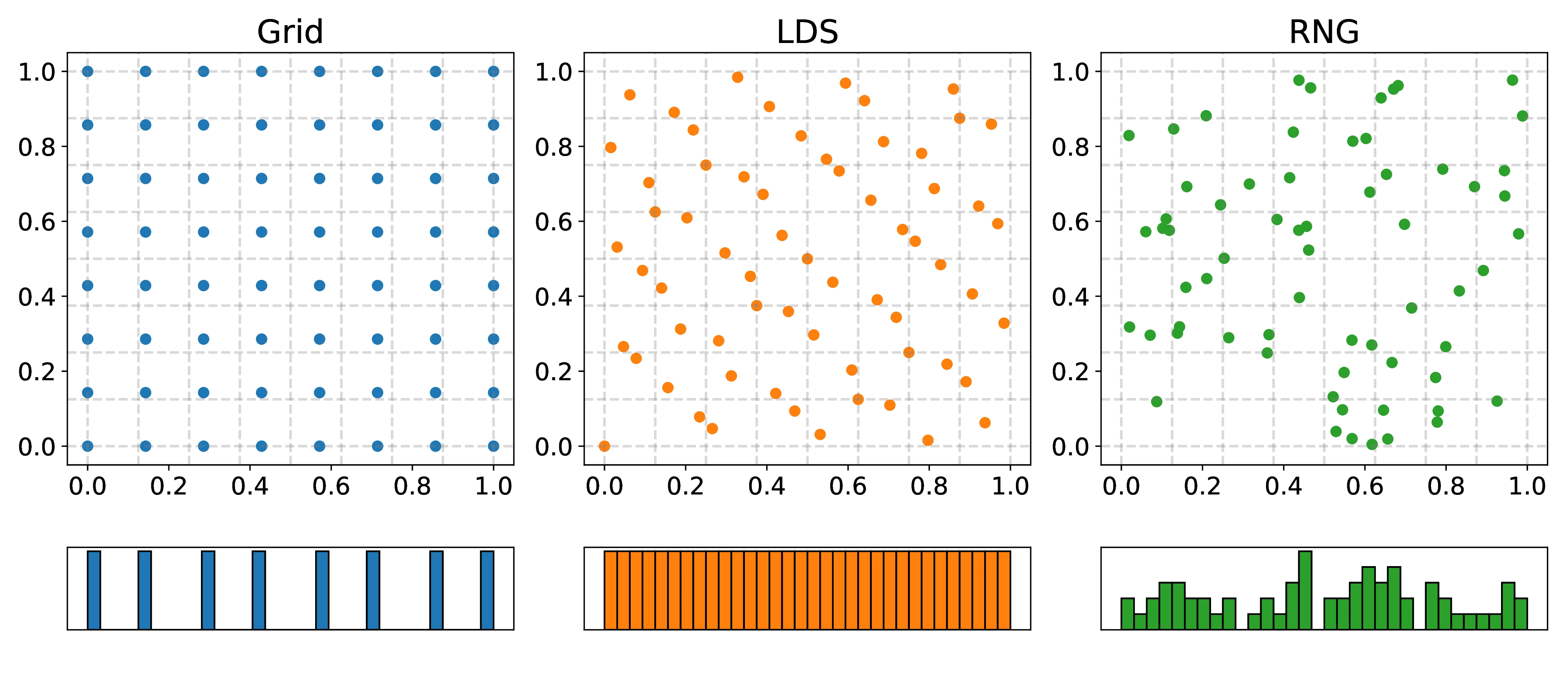
While being a key feature of Sobol and other low discrepancy sequences, such stratification properties are not unique to them. To illustrate, consider Figure [1] which divides the unit square into a grid. The left-most plot shows that deterministic quadratures like the trapezoid rule discussed above also stratify the unit square. Comparatively, the lack of stratification of (pseudo)random sequences can be seen on the right, where some of the boxes have an excess number of points while others are empty. Another feature of the plot is the projections of the sequences onto 1-dimension at the bottom of each figure, shown as histograms. Here, we observe the benefit of the `LDS` sequence relative to the `Grid` scheme where all points in a given axis project onto the same coordinate in 1-dimension, thus reducing the `effective` number of points. On the other hand, the `LDS` points have distinct values and thus do not suffer from this problem, as can be seen by the uniform histogram.
Before considering numeric properties calculated from Sobol sequences, we can consider properties of the direction numbers used to initialize a given sequence. As the direction numbers used to initialize the recurrence relations determine how the sequence is generated, their properties can influence the quality of the resulting sequence. Initially formulated in [17], properties A and A` properties represent uniformity conditions [16] that determine how the points in the sequence stratify the unit hypercube.
Definition 6 Property A [6]
A d-dimensional Sobol sequence with points satisfies property A if any binary segment of the unit cube, obtained by diving in half the unit hypercube along each dimension, contains exactly one point from the sequence.
Definition 7 Property A` [6]
A d-dimensional Sobol sequence with points satisfies property A` if any binary segment of the unit cube, obtained by diving by four the unit hypercube along each dimension, contains exactly one point from the sequence.
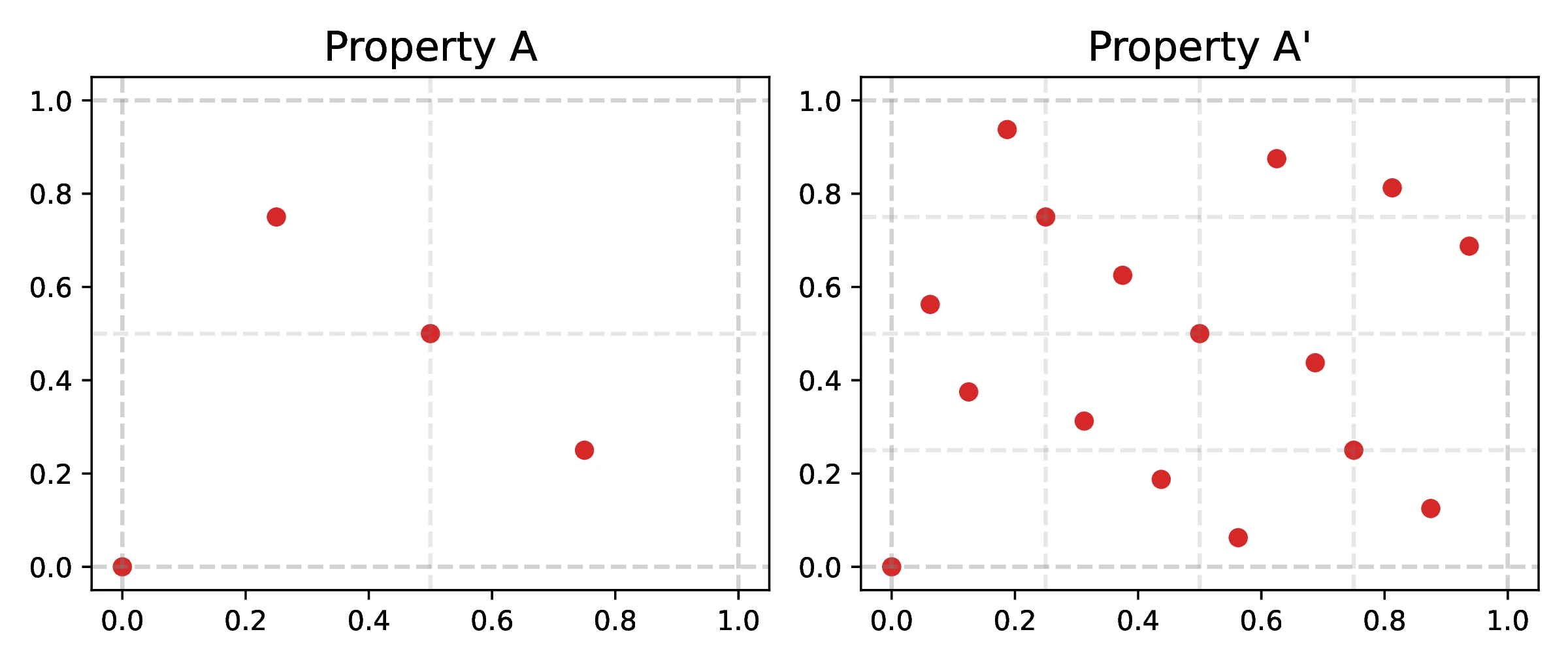
Points from a two-dimensional Sobol sequence satisfying both properties A and A` are shown in Figure [2], where one can observe that there is a single point in each subinterval. Thus, properties A and A` can be related to stratified sampling schemes, used for variance reduction [23].
Property A
A d-dimensional Sobol` sequence posesses Property A if and only if:
Where the matrix and is given by:
Here, the binary values denote the binary digit of the direction number for the dimension , where the entire direction number is represented by .
Property A`
A d-dimensional Sobol` sequence posesses Property A` if and only if:
Where the matrix is given by:
Similarly to Property A, the binary values represent the binary digit of the direction number given by: .
Properties A and A` in adjacent dimensions
In the case when the dimensionality, , of the Sobol sequence is large, we may choose to impose properties A and A` on a subset of the dimensions. One such choice can be subsets of variables forming a consecutive sequence, such that the dimensions satisfy and/or . These `adjacency` properties generalize and into and , with the former being special cases where . Such a generalization is useful when attempting to construct Sobol sequences in practice in order to reduce the search algorithm time complexity, while satisfying and/or only in adjacent dimensions. For a more in-depth discussion of and , see [1].
Given that the conditions for properties A and A` can be satisfied independently, a given sequence can satisfy both/one of/neither of these properties. As mentioned above, when searching for practical sequences, we may choose to utilize any combination of and , as well as potentially different values of . This affects the algorithmic complexity through the size of the determinants of direction numbers we need to compute.
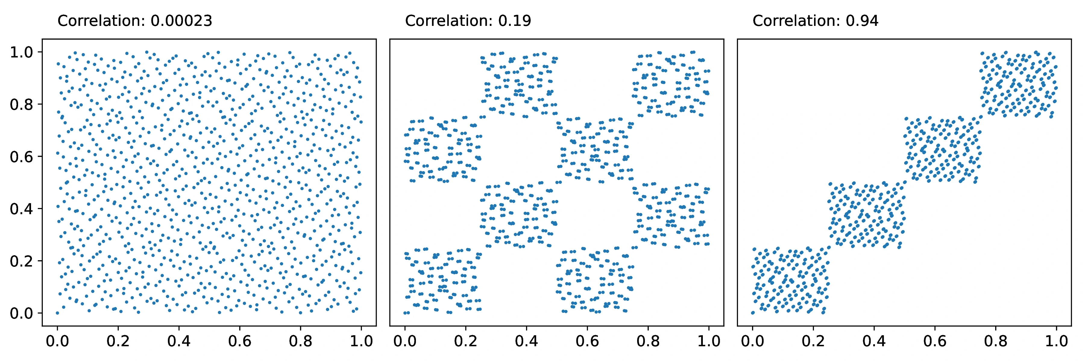
Although the properties described above are useful theoretically, we must also consider practical sequence equi-distribution properties for finite numbers of samples. While univariate Sobol sequences are always well distributed, higher dimensional sequences may exhibit significant co-dependence between individual dimensions for a finite number of samples. This can be illustrated by considering two dimensional projections of multidimensional Sobol sequences (Figure [3]), where we can contrast a well distributed two dimensional projection in Figure [3]a with two highly co-dependent projections showing in Figure [3]b and [3]c. Aside from filling the space non-uniformly, the poor equidistribution of the points lead to integration errors as some regions in the integration domain are completely empty. While increasing the number of points will asymptotically fill in such regions, these asymptotes will occur for impractically large samples. Thus, it is desirable to design sequences without such pathologies in the first place. One practical measure of the quality of the two dimensional projections is the Pearson correlation coefficient which we can compute after transforming each one-dimensional sequences through the inverse cumulative Gaussian distribution. Using this, we can quickly estimate the quality of the two-dimensional projections in the multidimensional sequence. We can construct a metric to minimize using this estimate, such as the maximum absolute correlation, that can be used when searching for direction number sets with the aim of generating sequences with improved projections.
While the two-dimensional projection evaluated at a low sample counts may show high correlations, a simple approach to reducing them, without searching for an alternative low discrepancy sequence, is to simply increase the number of points sampled - in the limit as the number of points the sequence discrepancy tends to zero. This space is filled uniformly and thus the correlations go to zero as well.
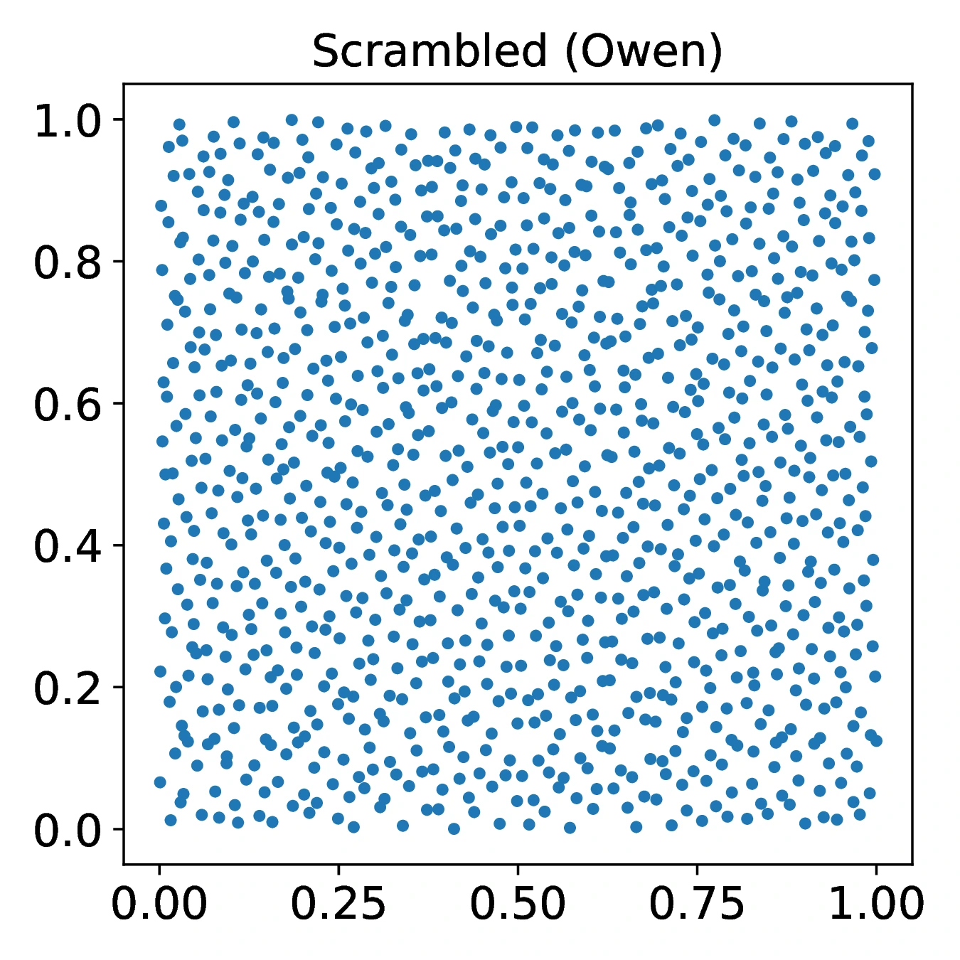
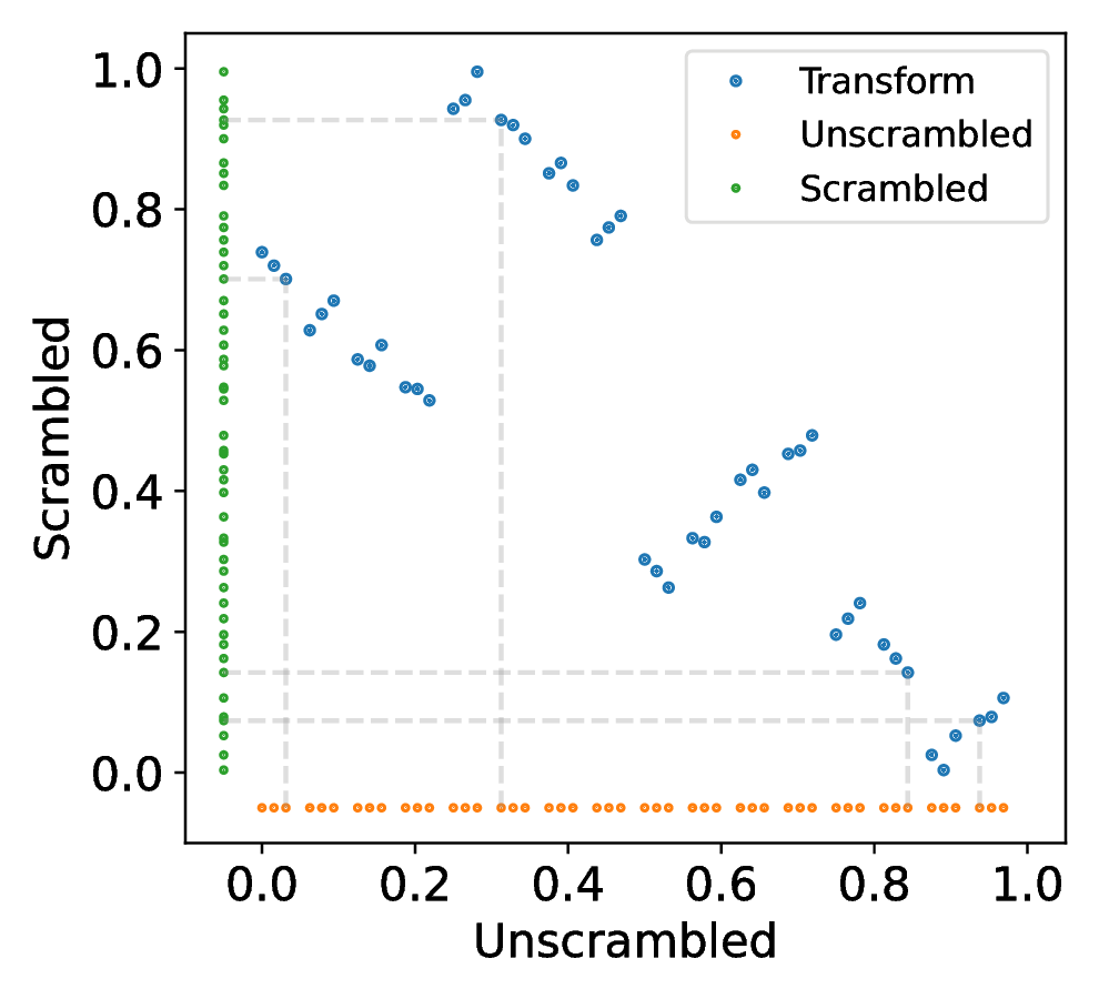
An alternative approach to reducing, but not eliminating, correlations is to scramble the individual one dimensional sequences using a method like Owen`s scrambling (see Section [3]). This preserves the discrepancy of the sequence and shifts the distribution of correlations towards lower values by permuting the elements of a given univariate sequence (Figure [7]). Being based on permutations of the unit interval, the scrambling method is thus unlikely completely wipe out all pathological two-dimensional projections, but one would expect it to improve the overall quality of the multidimensional sequence.
In this section, we describe two mathematical operations that need to performed when generating low discrepancy sequences: direction number generation and determinant calculation. Direction number generation involves mapping any integer to a direction number list, while determinant calculation is used to ascertain whether the direction numbers satisfy properties A and A`. We provide the theory and mathematical formulation for these concepts here and refer to them in section [Sequence: tkrg-a-ap5 (this work)] when searching for direction numbers.
To understand the process of direction number generation consider that they form an ordered sequence. A consequence of this is that there exists a mapping that converts the index of the sequence into the corresponding set of direction numbers. To help explain this we begin by considering integer sequences and their representation in an arbitrary in-place system like binary or decimal. When using such `in-place` systems a number is written as a sequence of digits in some base. The `base` assigns a possible number of values that a given digit can take. For example, every binary digit can take on either 0 or 1, every decimal digit can take on any value in {0,1,2...9}.
For common systems each digit has the same number of values, so the digit denoting the number of 10`s (in base 10) can take on the same number of values as the digit denoting the number of millions (). For a given base , we denote as the number of combinations for the digit, with . A given number with digits in base then consists of the following digits combination values:
The total number of possible combinations this digit string can represent is . In the example of base 2 with bits, we get . The number of combinations relates to how a number can be represented in the base. Consider the binary system again:
Denoting the powers of as allows the product to be represented as:
Where . For the case of the binary system, this means that the term is:
Where we define to make . In this way, we can represent a given integer using a non-constant base system, where the base of a given digit is . Using this, we can then represent the coefficients of the number by computing:
Counting with direction numbers
Consider the recurrence relation 3.6 of [1]. To be able to construct a given Sobol sequence using direction numbers (where denotes the position of the direction number in the dimensions sequence, and denotes the dimension), we need a total of initialization direction numbers: . These direction numbers can be obtained from their integer representation . For a given position , the corresponding direction number must satisfy:
is odd.
Thus, for the position , there are possible direction numbers . The number of coefficients is therefore calculated using the following equation:
Hence, we can view the generation of direction numbers as decomposing a given number into a non-uniformly sized digit representation with the number of combinations per digit given by . Using this method, we can construct functions that map a given number onto a corresponding direction number list by treating each of the direction numbers as a digit.
A Galois field consists of only two elements , and defines the following addition () and multiplication () operators:
| \ | |||
|---|---|---|---|
| 0 | 0 | 0 | 0 |
| 0 | 1 | 1 | 0 |
| 1 | 0 | 1 | 0 |
| 1 | 1 | 0 | 1 |
While this appears to be a trivial modification to standard addition and multiplication defined on the real numbers, the consequences of this for the calculation of determinants in high dimensions and on computers are profound. The first of these is the ability to use one bit per matrix element giving a per-element memory reduction. This allows us to represent a larger matrix in using the same memory, compared to a 64-bit floating point number. The second set of consequences relates to the algorithms for calculating determinants; we must modify these to account for the new arithmetic. In python, this can be done by casting numpy matrices to contain elements in GF(2) using the `galois` python library. There are other aspects of GF(2) matrices that are more mathematical. The first of these is that in GF(2) there are vectors of elements which are self-orthogonal, i.e. when . To illustrate, consider the following:
In addition, for a random matrix of elements, the probability that the matrix is non-singular (has a determinant = 1) is given by [24]:
Taking the limit as , the probability of finding a non-singular matrix at random tends to [24]. This contrasts with the case for random matrices with elements in , where the probability of finding a singular matrix tends to ; high dimensional random vectors become approximately orthogonal. Thus, the problem of finding a non-singular matrix is comparatively harder for GF(2) than for . However, it may still be possible to find a non-singular matrix within a tractable number of attempts.
Low discrepancy sequences (LDS), unlike random numbers, are deterministic and thus unable to provide a standard error on the estimate due to the non-applicability of the CLT. This is problematic as we are then unable to quantify the uncertainty around the estimate. Additionally, problems might arise when a `bad` number of points in a given sequence is used. While we can simply add a random number to each point of the sequence, this would increase the discrepancy of the resulting sequence. Hence, the challenge is to restore `randomness` (for the purposes of applying the CLT) without sacrificing the low discrepancy of the sequences (and by proxy - the convergence rate of the estimator). This can be achieved with `Randomized Quasi Monte-Carlo` where we apply a `scrambling` operation to the low discrepancy sequences. A good scrambling operation (defined by the `seed` parameter) will map the input LDS to another LDS with sufficient `randomness` to allow the computation of a standard error estimate. This is because scrambling the sequence with different seeds allows the application of CLT. Moreover, a good scrambling algorithm may also help reduce the non-uniformity of the Sobol sequences.

The simplest method for scrambling a low discrepancy is simply adding a uniform random number separately to each of the d-dimensions. This is known as a Cranley-Patternson (CP) rotation [23].
The rotation preserves the low discrepancy nature of a sequence (Equation \ref{eq:cranley_patterson_discrepancy}), but does not eliminate pathological non-uniform regions in the sequences; it merely shifts them. As the shifts are continuous, the CP rotation also does not preserve the stratification properties of the digital sequences achieved by subdividing the unit hypercube.
Digital scrambling is a similar operation to the CP rotation described above. However, here we work with the integer representation of the low discrepancy sequences, performing instead a summation in base-b between values in each dimension of the sequence and the uniform number:
Representing both the low discrepancy value and the scrambling value in base-b where an arbitrary value can be written as:
The per-digit scrambling operation can then be expressed as:
For the case of Sobol sequences, the base-2 operation summation is the XOR making it fast to compute on modern computers. Similar to the CP rotation, a key downside of digital shift scrambling is that they do not randomize the sequence sufficiently, and thus do not achieve a significant improvement of estimate variance properties.
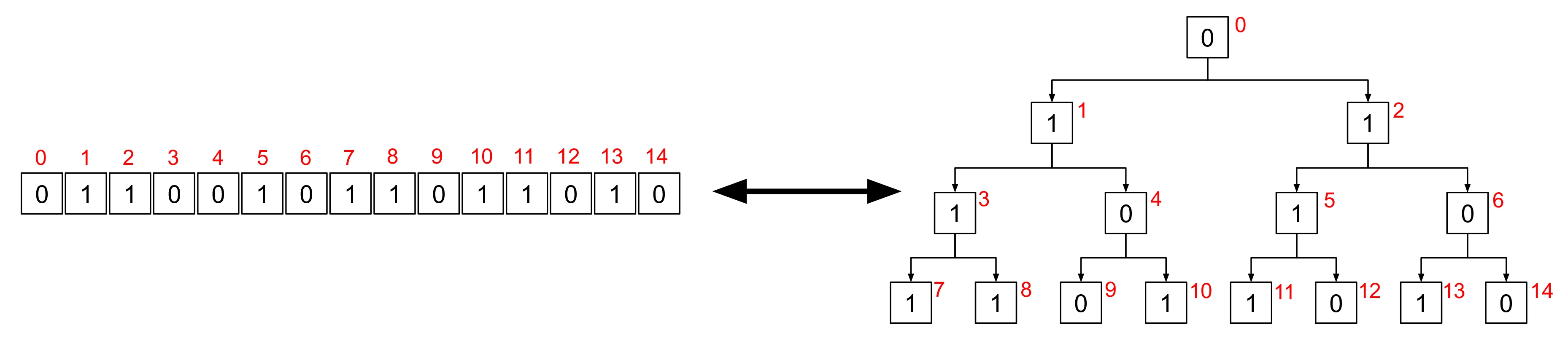
A more powerful approach to randomization is Owen`s scrambling, also known as nested uniform scrambling. Like the previous scrambling methods, Owen scrambling applies to each dimension separately. Within each dimension the nested uniform scrambling can be viewed as an extension of the digital scrambling where the bits of a number are XOR-ed with bits of a scrambling sequences. However, unlike digital scrambling where the scrambling sequence is constant, the scrambling sequence is sampled in a path-dependent way from a set of random bits generated for the scrambling. To illustrate with an example, consider the following binary sequences of length :
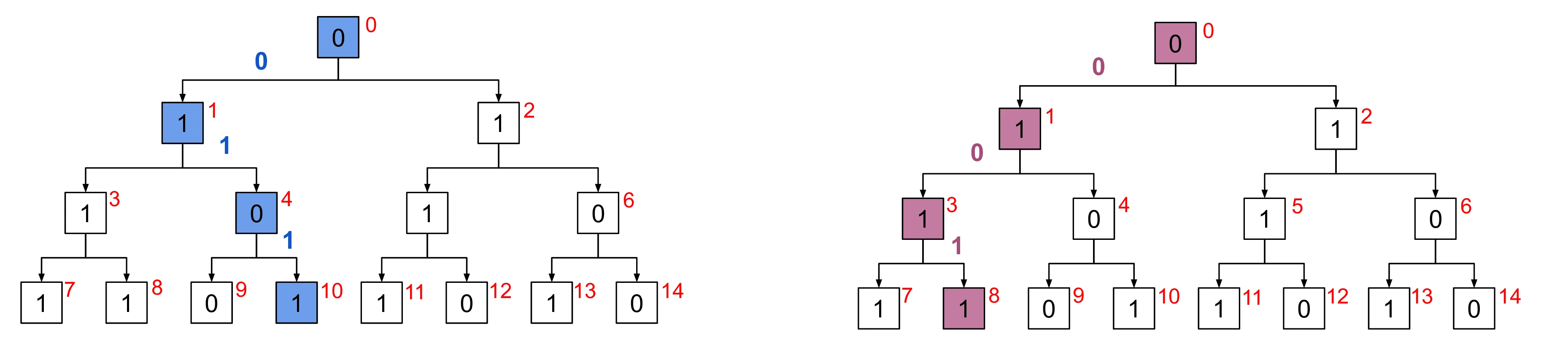
Generation of scrambling sequences for these requires a random values which can be interpreted as forming a binary tree, as shown in Figure [5]. Given this binary tree, we can generate scrambling sequences for and by traversing the binary tree, taking the left branch when we encounter a in the value of (or ) and right when we encounter a . Examples of this sort of tree traversal are shown in Figure [6].
The scrambling sequences generated by traversing the binary tree for and are:
The path through the binary tree used to obtain these scrambling sequences is shown in Figure [6] which highlights the nodes of the binary tree that make up the digits of each value of . The edges of the binary tree are annotated with the digits of the scrambled value (/) to show how this path through the tree was obtained.
Having generated the scrambling sequences we can now calculate the resulting scrambled values using digital scrambling:
Formally, nested uniform scrambling can be viewed as a path-dependent permutation of the intervals. In this way, the scrambling rearranges the sub-intervals, but does not change the number of points in each sub-interval, thus preserving the uniformity properties. In this context, the source of randomness is the binary tree - defining the permutations to be performed. A key limitation of Owen`s scrambling is that for a d-dimensional Sobol sequence with a scrambling depth of in base-b, the scrambling requires values in order to store the binary trees for each dimension. Thus, scrambling 32-bit Sobol sequences requires MiB/dimension. Practical techniques for reducing memory usage are to limit the scrambling depth to bits and apply a digital scramble to the remaining digits. An alternative is to approximate a binary tree with a hash function to scramble the bits.
The hash-based Owen scrambling replaces an explicit binary tree used to calculate the scrambling bit with an implicit traversal - a hash function. Here, instead of traversing down the tree we note that, for a given bit, the previous bits form a path or address of the next random bit to XOR with the bit being scrambled. Thus, to scramble a given bit of , we use the preceding bits: we can treat the binary tree as a scrambling function into which we pass this address. Replacing the binary tree by a hash-function we can get the effect - the next random bit. To emulate randomness, we replace the RNG used to generate the binary tree with a random seed, also passed into the hash function. Hence, to compute the random bit that is then XOR`ed with the input bit to generate the scrambling, we perform:
A naive implementation would iteratively apply this formula to perform a nested scrambling. However, applying a per-bit hash function is computationally expensive. An alternative approach described in [8] and based on the Laine-Karras (LK) hash function [9]. This hash function approximates the set of bit-wise hash calculations and vector XOR operations in one go, improving efficiency. Finally, the LK-hash must be applied to Sobol values in reverse order starting from the least significant bit. With this, the LK-hashing becomes a good approximation to Owen scrambling, permuting the elementary intervals and retaining the good stratification properties \\cite{building_better_lk_hash}.
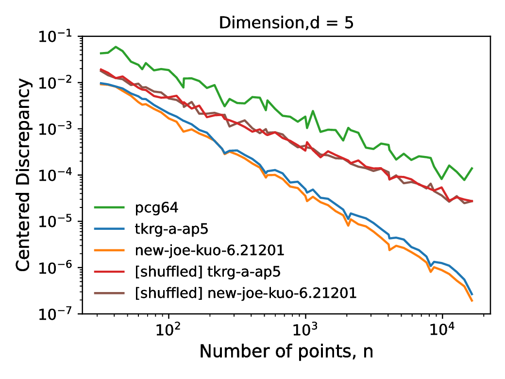
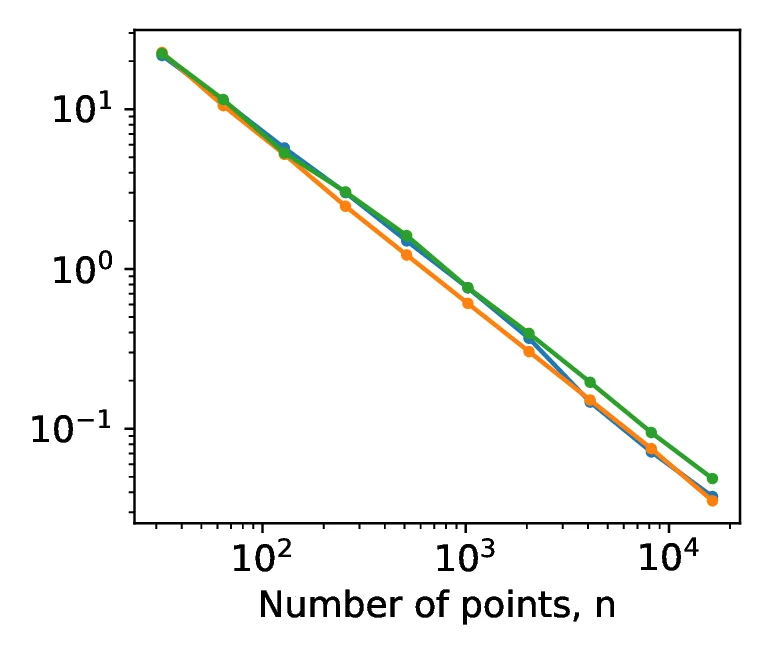
While scrambling acts on the values of a points in the sequence, shuffling acts on the index (the order), reordering them without changing the values. This approach, described in [8], is aimed solely at reducing the correlations between dimensions, as opposed to scrambling which aims to improve sequence properties. While [8] described a `nested uniform shuffle`, our implementation utilizes a random shuffling to remove the correlations between individual one-dimensional Sobol sequences within the multidimensional sequence. As the one-dimensional points remain unchanged by the shuffling, the distribution of the points remains unchanged. However, as shown in Figure [8], the shuffling degrades the scaling of discrepancy with increasing point count for higher dimensions. The relation, on a log-log scale, between the centered discrepancy and number of points, , is described by the formula:
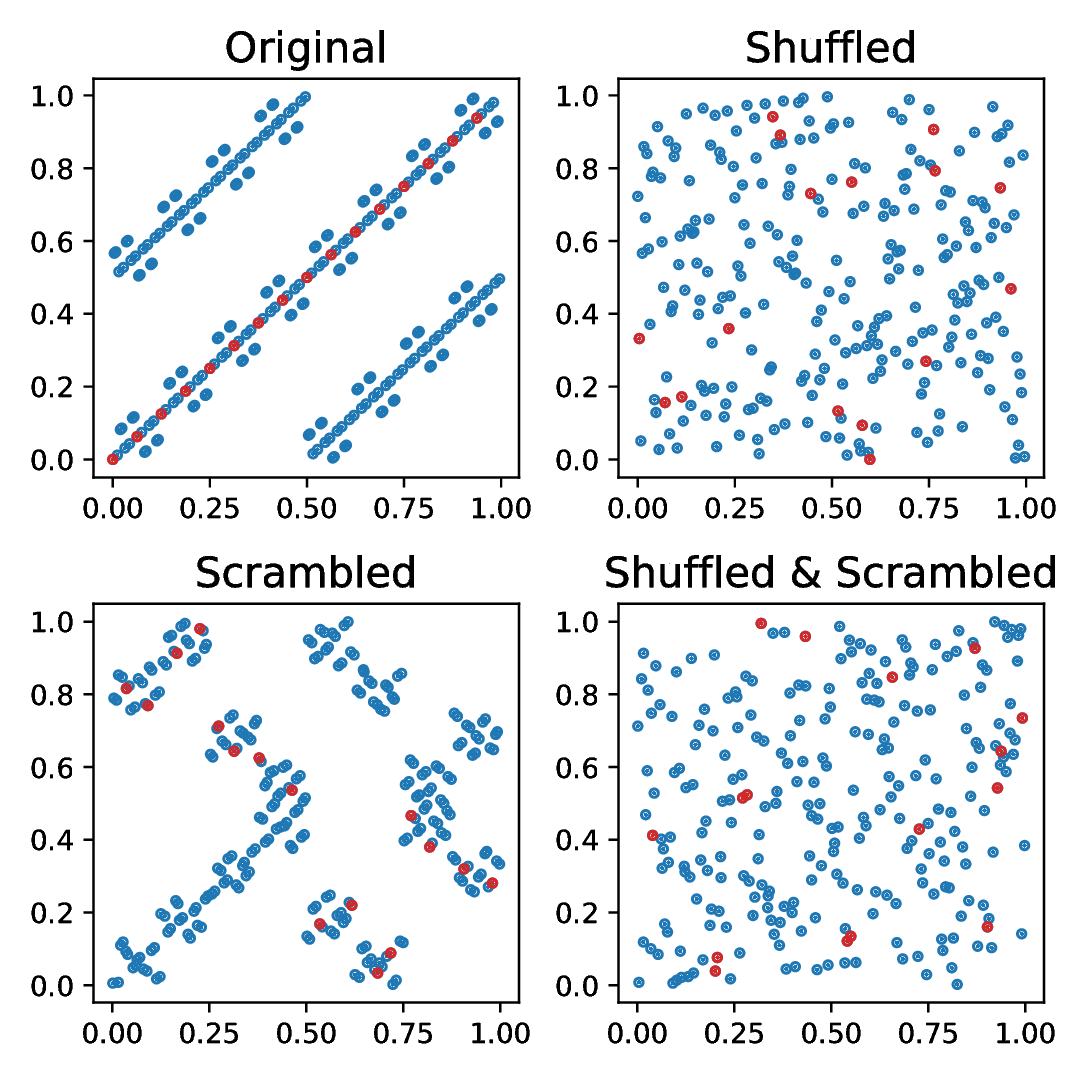
Prior to shuffling, the gradient, , of the tkrg-a-ap5 and new-joe-kuo-6.21201 were and respectively. Meanwhile after shuffling, the new values of are and , significantly closer to that of the pcg64 generator, at . This acts to illustrate that by shuffling the sequence we can decorrelate the individual dimensions, but at the cost of reducing the high dimensional equidistribution properties. An example of how scrambling and shuffling influence the two dimensional projections is illustrated in Figure [9] which illustrates that we can decorrelate individual dimensions by shuffling and scrambling, and thus achieve both randomization and decorrelation by combining the techniques.
To evaluate the quality of the directed numbers generated by the search procedure outlined above, we compare the performance of the generated Sobol sequences with the new-joe-kuo-6.21201 direction numbers described in [22],[4], using pseudo-random sequences generated by the pcg64 [10] as a baseline. In the following section, we present the key findings of our benchmarking, while the full set of test integrals and discrepancy measures is included in Appendix [C]. We note that low discrepancy sequences are expected to outperform pseudo-random numbers in the case when the test problem has a low `effective` dimension (distinguishing it from the `nominal dimension` of a problem - the number of terms in the integral). Thus, we plot a mean dimension of the test problem alongside the test metric where applicable to allow the reader to verify the suitability of applying low discrepancy sequences. Discussion on mean dimension alongside the relevant formulae are presented in the Appendix [A].
The approach employed by Joe and Kuo for searching for new direction numbers accounts for the fact that property A is not sufficient to prevent correlations between pairs of dimensions (we denote dimension as ). Joe and Kuo, therefore, take advance of the fact that a Sobol sequence can be viewed as a -sequence in base 2, where every block of points forms a -net. Hence, the -value, given by ,, can measure the uniformity of point sets; smaller -values lead to finer partitions, and hence more uniformly distributed points. Using the aforementioned concepts, Joe and Kuo adopted the following method:
Search for direction numbers that satisfy property A for dimension 1,111 by assigning polynomials for each dimension up to degree 13.
After 1,111 dimensions, search for direction numbers that optimize the t-values of the two-dimensional projections, reaching 21,201 dimensions.
Joe and Kuo made the following assumptions when defining their search criterion: direction numbers were already chosen up to dimension and that is given and fixed. They would thus aim to choose direction numbers for dimension so as to minimize the t-value.
Similarly to [1], our search strategy to generate tkrg-a-ap5 was to search for Sobol sequences satisfying the following properties:
Property A for all 195,000 dimensions ()
Property A` for 5 adjacent dimensions ()
The reason for choosing to search only for is Lemma 2 of [1] which states that it is not possible to construct a Sobol sequence for satisfying for all . In order to obtain Sobol sequences which satisfy properties A () and A` (), we needed to find sets of direction numbers whose digits satisfy the equations \ref{eq:property_A} and \ref{eq:property_Ap}. In [1], the suggested proposal appeared to formulate this as a set of constraints, in effect transforming this search into a satisfiability problem - solvable by automated theorem provers. A potential benefit of this approach is to generate all possible direction numbers satisfying the given constraints. However, such boolean satisfiability is in general NP-hard. Instead of this the key to our approach is the efficient calculation of the determinants of high-dimensional matrices in the Galois field GF(2) (Section [Determinants in GF(2)]).
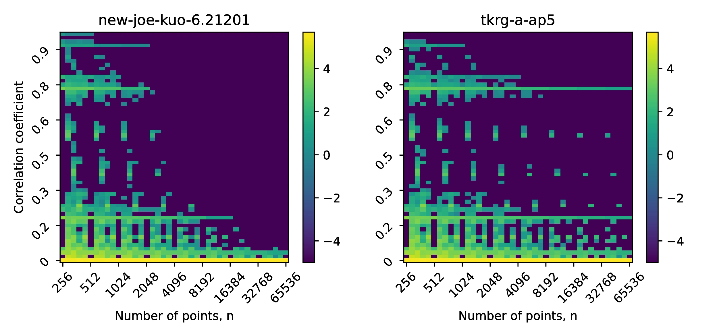
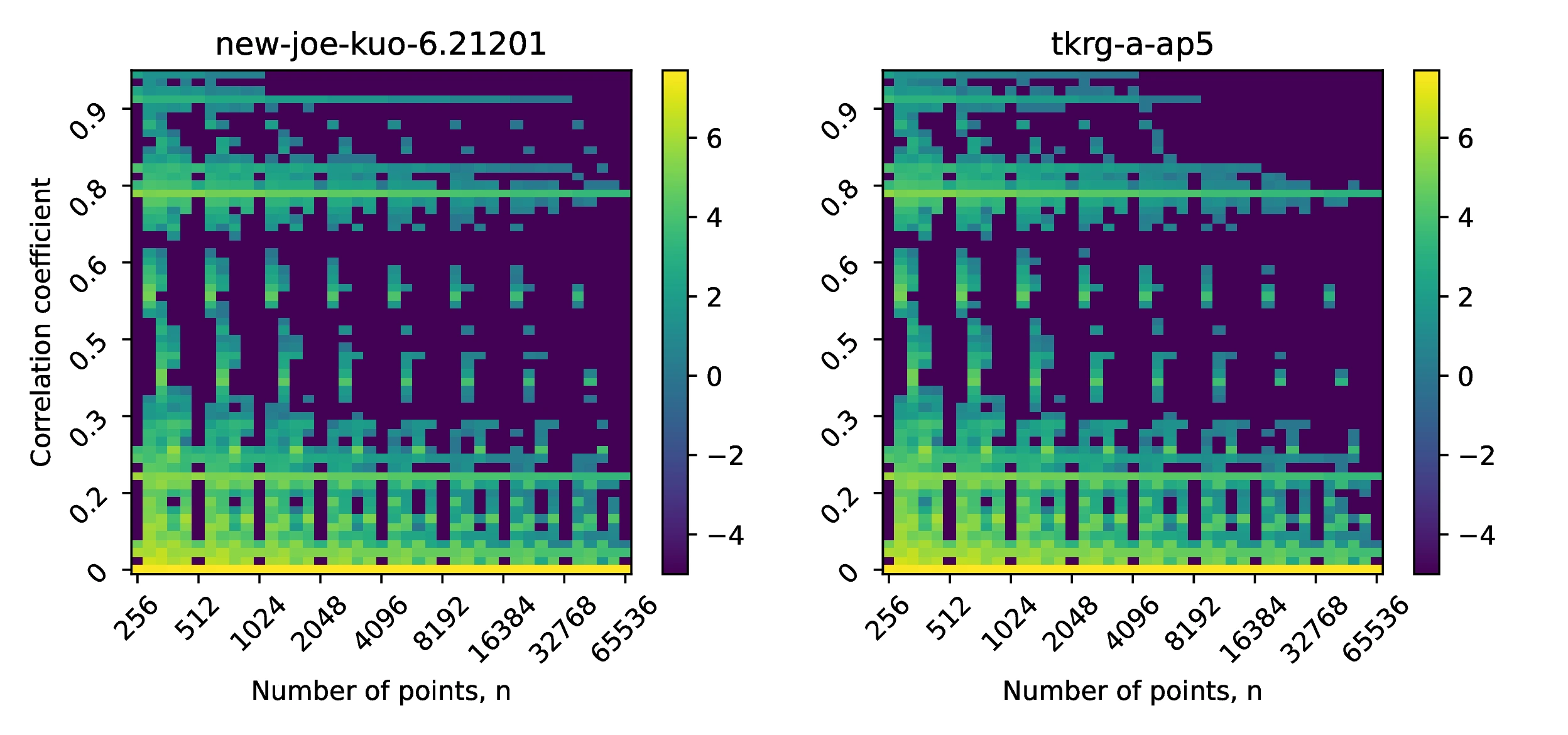
One of the factors that could affect the uniformity properties of tkrg-a-ap5 is the correlation between dimensions. To investigate the effect of the numper of sampled points in the sequence, we compare the correlation coefficient histograms in two dimenions for the first 1,000 ([10]a) and 10,000 ([10]b) dimensions of the new-joe-kuo-6.211201 and the tkrg-a-ap5 sequences. We show the heat maps of both sequences in Figure [10]. In both cases, we observe that as the number of points `n` increase, the distribution of correlation coefficients shifts towards zero. This is most apparent for the new-joe-kuo-6.211201 direction numbers in the case of 1,000 dimensions. The figures also help to illustrate that choosing an `n` arbitrarily, instead an integer power of 2, produced unbalanced point sets - increasing the number of highly correlated dimensions unnecessarily.
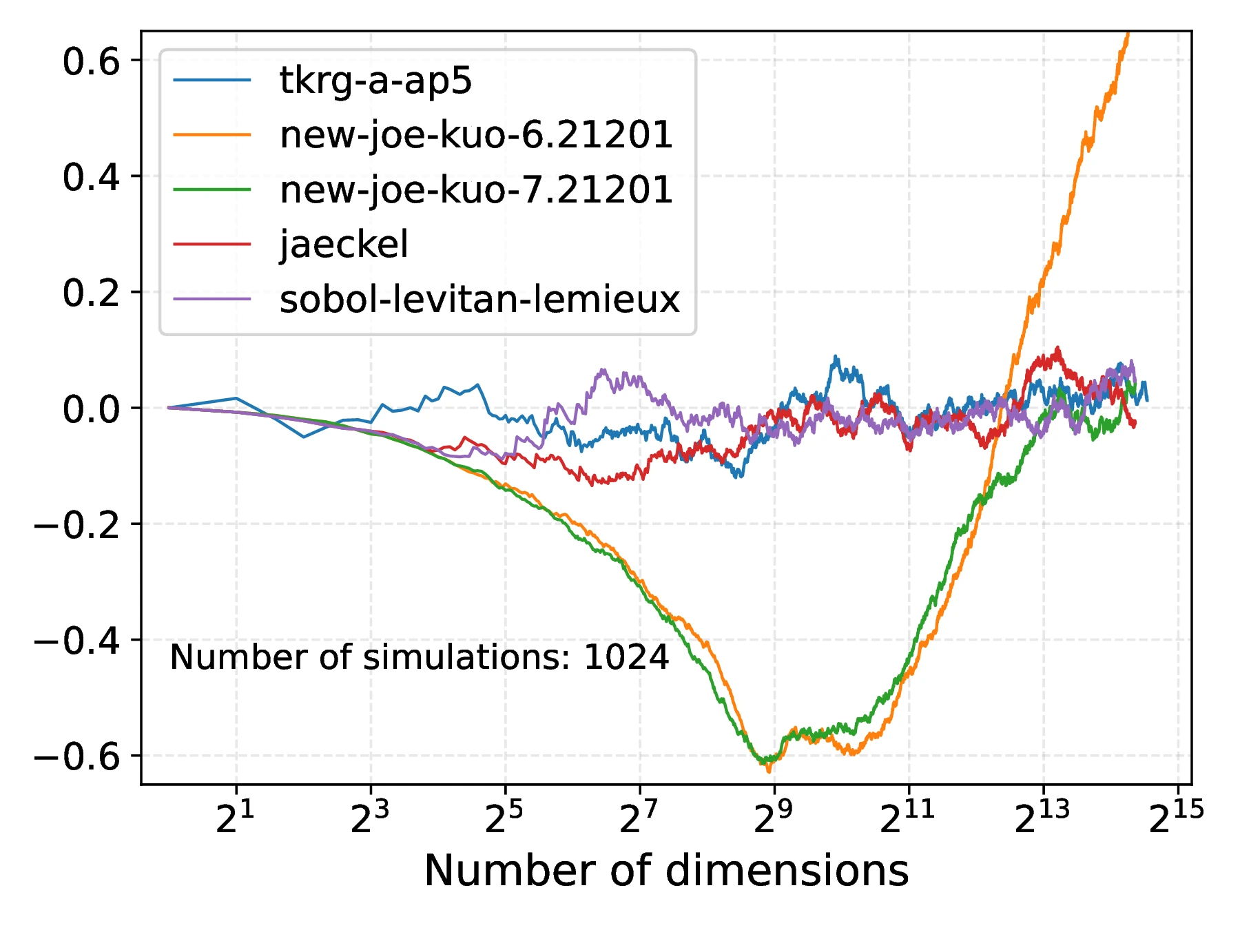
Here, we examine the spurious variance of a multidimensional Sobol sequence. This quantity is a measure of the the average pairwise correlation between dimensions of a Sobol sequence (see Appendix Section [B] for full description) and is given by:
Plotting against dimensions in Figure [11]a, we observe that the tkrg-a-ap5 direction numbers exhibit substantially less deviation from zero than the new-joe-kuo-6.21201 sequences. This may be attributed to the increased uniformity of the tkrg-a-ap5 sequence that gives rise to a more symmetric distribution of correlation coefficients, in turn resulting in the maximum deviation of the spurious variance being smaller. In contrast, the new-joe-kuo-6.21201 sequences have consecutive sets of correlation coefficients whose distribution is highly asymmetric (around zero), thus resulting in the spurious variance drifting away from zero until approximately . This behaviour of having highly biased distributions of correlation coefficients between dimensions appears to be a feature of the new-joe-kuo-6.21201, as other sequences such as sobol-levitan-lemieux or jaeckel do not exhibit such deviations; such a structure may have arisen as a result of the employed direction number search strategy used in [4] to generate the sequence.
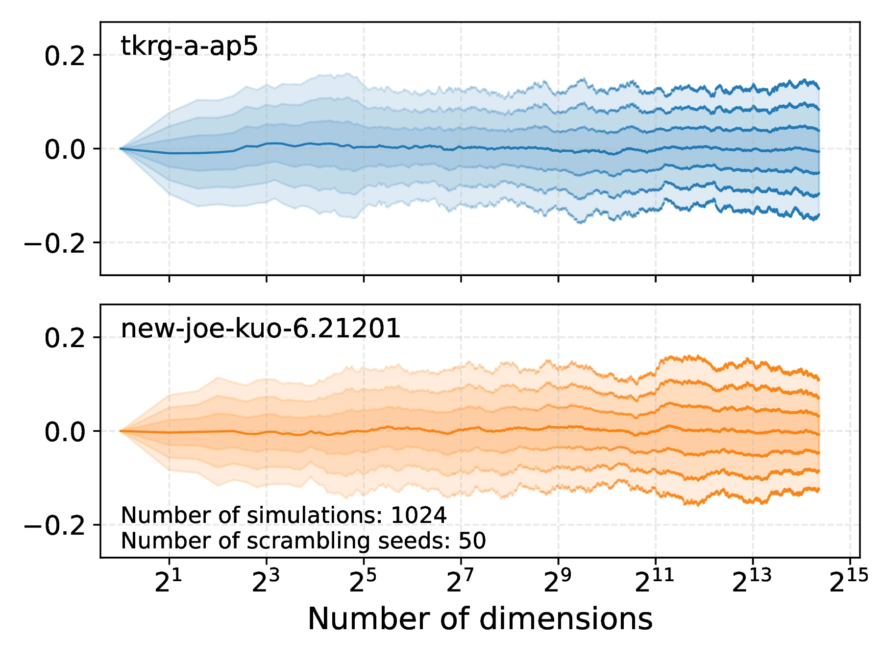
An effective strategy to decorrelate and make symmetric the correlation coefficient distribution is to scramble the underlying low discrepancy sequence, before recomputing the spurious variance for each scrambled sequence. The effect of this is shown in Figure [11]b where the mean, obtained by averaging 30 spurious variance traces, of both the tkrg-a-ap5 and new-joe-kuo-6.21201 are shown - with the latter no longer exhibiting the large drift away from zero, present in Figure [11]a.
A second method for assessing quality of the low discrepancy sequences is to evaluate numerical integrals, whose value can be calculated analytically, and comparing the results obtained (see Appendix [C] for a full comparison of test integrals). Here, one considers the absolute error between the numeric and analytic result against the number of points used, as well as other parameters like dimension of the integral or other terms in its definition that can affect its difficulty. Unlike with Monte-Carlo, in the case of QMC we cannot rely on the central limit theorem, and thus must know analytic results to measure convergence. Using randomization (RQMC), we can attempt to recover the ability to estimate the error using the CLT. However, we must compute multiple scrambled versions of the sequence - increasing the computation time.
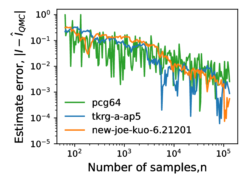
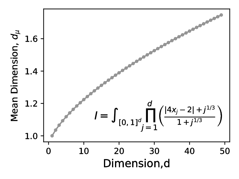
Consider first the integral below. Its integrand is a product of individual dimensions , with being the nominal integral dimension and being a constant term, parameterized by the index of the dimension . We can scale the integrals difficulty, its effective dimension (see Appendix [A]), by setting which determines the size of the denominator relative to the numerator of each of the product terms.
In [21], the authors discuss three variants for , a constant , a quadratic and a partial power dependence . In all cases the analytic solution is . However, the integrals have different effective dimensions, with the quadratic scaling having the lowest effective dimension for a given actual dimension . In Figure [12], we consider the first case, with for , where we show that the error of QMC does not appear to decay at a faster rate that of MC, represented by the pcg64 line. This may be attributed to the form of the product terms, where each term contributes equally to the effective dimension - albeit with a scaling coefficient of , meaning that each nominal dimension contributes only slightly to the effective dimensionality. Of the three cases considered, convergence benefits of low discrepancy sequences for test integral are observed only for the case of , where the effective dimension tends to as the nominal dimension .

A second test integral , also considered in [21], is defined as:
Here, the decay of each nominal dimension to the mean effective dimension (in the multiplicative superposition sense) is similar to the case of with thus the contribution of successive nominal dimensions decays to zero with increasing dimension index. Consequently the effective dimension for tends to an asymptotic value of as , as shown in Figure [13b]. The result of this small value of effective dimension gives rise to the fast onset of the convergence rate, shown in Figure [13a].
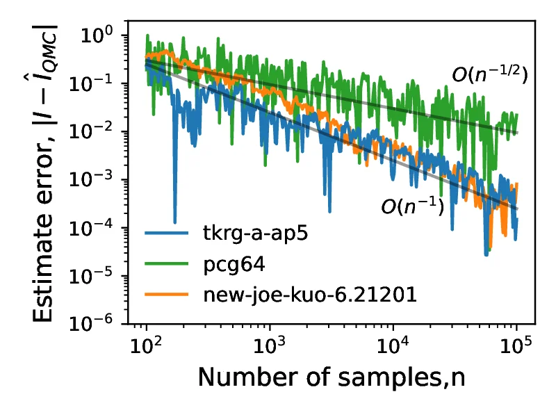
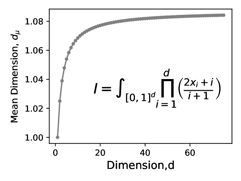
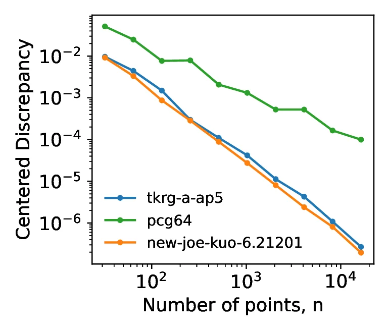
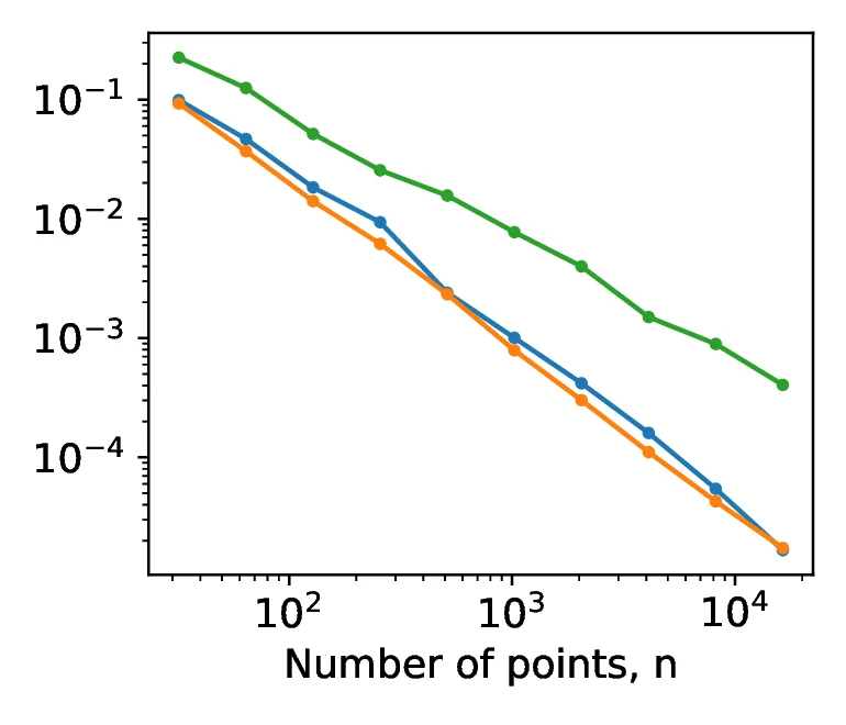
Figure [14] shows plots of centred discrepancy versus number of points for the tkrg-a-ap5, new-joe-kuo-6.21201 and pseudorandom sequences at dimensions 5, 10 and 30. For all dimensions and sample sizes, the performance of tkrg-a-ap5 and new-joe-kuo-6.21201 are similar. The pseudorandom sequences are the worst performing on dimensions 5 and 10, while the convergence rate of the pseudorandom sequence at dimension 20 is similar to that of tkrg-a-ap5 and new-joe-kuo-6.21201.
In this report, we reviewed the basic theory of low discrepancy sequences and the conditions under which such they can be applied to Monte-Carlo numeric integration. When applied to suitable problems, the Quasi-Monte Carlo methods estimator convergence rates of , converging faster than conventional Monte-Carlo which exhibits an rate. We then considered Sobol sequences which are base-2 low discrepancy sequences, defined using recurrence relations from an initial set of direction numbers and primitive polynomials. We showed that when sampling, it is critical to keep the number of points in a sequence a power of 2, required to maintain `balanced` sequences, in maintaining the improved convergence rate and minimizing bad two-dimensional projections quantified by computing correlation coefficients. We then presented properties A and A`, relating them to properties of the direction numbers and outlined a strategy to search for such direction numbers by performing determinant calculations in GF(2) - allowing us to generate the tkrg-a-ap5 sequence. Following this, we covered Randomized QMC introducing three different scrambling techniques followed by presenting a comprehensive set of benchmarks for evaluating LDS sequences in both low and high dimension.
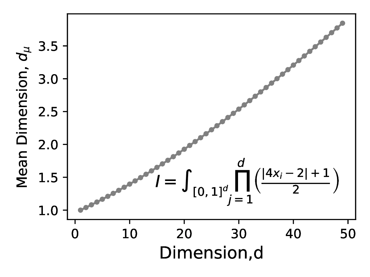
While the `nominal` dimension of (the integration domain) can give an indication of the difficulty of the integration problem, some integration problems may have a `effective` dimension that is significantly lower this nominal value. In this case, the majority of the contribution lies in a lower dimensional manifold, sampling from which we can converge to the target solution at a rate substantially faster than predicted by the nominal dimension. This class of problems is the one most suitable for QMC integration. Calculating an `effective` dimension in practice is challenging, but analytic equations exist for integrands that have a certain functional forms. Two forms, as discussed in [7] are given below. Example of function with these forms are shown in [3].
In the subsequent sections, we use the following terms:
: the dimensionality of the function;
: a subfunction applied the th dimension;
: the th element of a given random sample.
Integrands in the additive form can be represented as a sum of simpler terms:
The mean effective dimension of the additive function in the superposition sense is one:
The mean effective dimension of the additive function in the truncation sense is given by:
Integrands in the multiplicative form can be represented as a product of simpler terms as follows:
The mean effective dimension of the multiplicative function in the superposition sense is:
The mean effective dimension in the truncation sense is not defined.
In this section, we describe the `spurious variance` test used to evaluate quality of the low discrepancy sequences. In it we consider independent and identically distributed random variables . Performing a summation over sum variables, we obtain a new random variable :
In the case when the random variables satisfy the IID assumption, the resulting variance of reduces to:
While this equality will not hold exactly for finite sample sizes, it should hold approximately and can thus be used to check whether the samples generated are approximately independent and identically distributed. These assumptions may not hold in practice when the underlying number generators exhibit pairwise correlations between dimensions of the random numbers. Such correlations will give rise to an additional unwanted or `spurious` variance term - causing the sum of the random variable samples to deviate from the theoretically predicted value. Thus, by calculating this spurious variance term, we can assess the quality of multidimensional low discrepancy sequence due to the one-to-one mapping between random variables and the dimensions of the low discrepancy sequence.
Generalizing the above two variable sum to variables, and applying the bilinearity of covariance:
where and are scaling factors, while and are random variables drawn from a Gaussian distribution.
We can obtain the following expression for the variance of the sum :
Here, the second term is the pairwise sum of correlation coefficients running over all unequal indices , where again we have applied the reductions for all . In the case when the individual random variables are independent and identically distributed the correlations, for all . However, when the two dimension projections of the sequences exhibit non-zero correlations, the resulting correlations directly impact the variance , as . Thus, by computing variance of and measuring its deviation from the ideal case when for , we can detect problematic two dimensional projections in a d-dimensional sequence.
One way of comparing low discrepancy sequences is by estimating the error of various integrals and comparing these estimates to the analytic solutions of the same integrals. Given that the analytic solution of the test integral is known, the approximation errors and its rate of convergence (or lack thereof) can be used to assess the quality of the low discrepancy sequence, or other MC/QMC approach. In general the rate of convergence will depend both the sample generation method and the integral being estimated. By plotting the estimate error with increasing number of samples on a log-log plot and extracting the gradient one can then estimate the convergence rate. This is the topic of this appendix
Section [Classes of test integrals]: presents a table of test integrals with additive and multiplicative form (see Appendix [A]).
Section [Non-Decomposable test integrals]: presents several special integrals that have neither additive or multiplicative form.
Section [Experiments]: presents experimental results on some of the additive and multiplicative alongside a discussion.
The first set of integrals we examine are those that can be categorised as either additive or multiplicative. These categories refer to the means of decomposing the integrals: either as a summation or a product of several sub-integrals (one sub-integral per dimension). We provide the mathematical formulations of each category, as well as possible instantiations of the two classes in the following two tables. these integrals have analytic solutions against which the estimation error can be calculated. The sources of the test integrals are given in the right-most column of the second table. Additionally, is defined as the number of dimensions, is the sub-integrand for dimension and is the scaling factor.
| Name | Integral class | Functional form | Parameter values | Expected value | Reference | |
|---|---|---|---|---|---|---|
| hellekalek_function | Multiplicative | 1 | [7] | |||
| sobol_1 | Multiplicative | 1 | [7] | |||
| sobol_2 | Multiplicative | 1 | - | [7] | ||
| owens_example | Multiplicative | - | [7] | |||
| roos_and_arnold_1 | Additive | - | [7] | |||
| roos_and_arnold_2 | Multiplicative | 1 | - | [7] | ||
| roos_and_arnold_3 | Multiplicative | 1 | - | [7] | ||
| genzs_example | Multiplicative | 1 | [7] | |||
| subcube_volume | Multiplicative | 1 | = | [1] | ||
| high_dim_1 | Multiplicative | 1 | - | [1] | ||
| high_dim_2 | Multiplicative | 1 | - | [1] | ||
| high_dim_3 | Multiplicative | [1] | ||||
| high_dim_4 | Multiplicative | - | [2] | |||
| joe_kuo_1 | Multiplicative | 1 | - | [6] | ||
| lds_investigations_f1 | Additive | - | [3] | |||
| lds_investigations_f2 | Additive | - | [3] | |||
| lds_investigations_f3 | Additive | - | [3] | |||
| lds_investigations_f4 | Multiplicative | 1 | = | - | [3] | |
| lds_investigations_f5 | Multiplicative | 1 | [3] | |||
| lds_investigations_f6 | Multiplicative | 1 | - | [3] | ||
| lds_investigations_f7 | Multiplicative | 1 | - | [3] | ||
| lds_investigations_f8 | Additive | = | [3] | |||
| lds_investigations_f9 | Additive | [3] | ||||
| optimization_f1 | Additive | - | [5] | |||
| optimization_f2 | Additive | - | [5] | |||
| optimization_f3 | Multiplicative | 1 | - | [5] | ||
| optimization_f4 | Multiplicative | 1 | and | [5] | ||
| optimization_f5 | Multiplicative | 1 | and | [5] |
This section contains test integrals that are neither additive or multiplicative and whose integrands cannot be decomposed into sums or products of sub-functions for each nominal dimension. Nevertheless, such test integrals are also useful as decompositions of the integrands into sums or products is not guaranteed. Thus, in this section, we present non-decomposable integrals and discuss their characteristics. In addition to the absolute numeric estimate errors, we provide 3D projections of the surfaces where the difficulty of the integral can be assessed qualitatively. This is because there is no simple method of calculating the effective dimension, so the 3D projections act as a substitute.

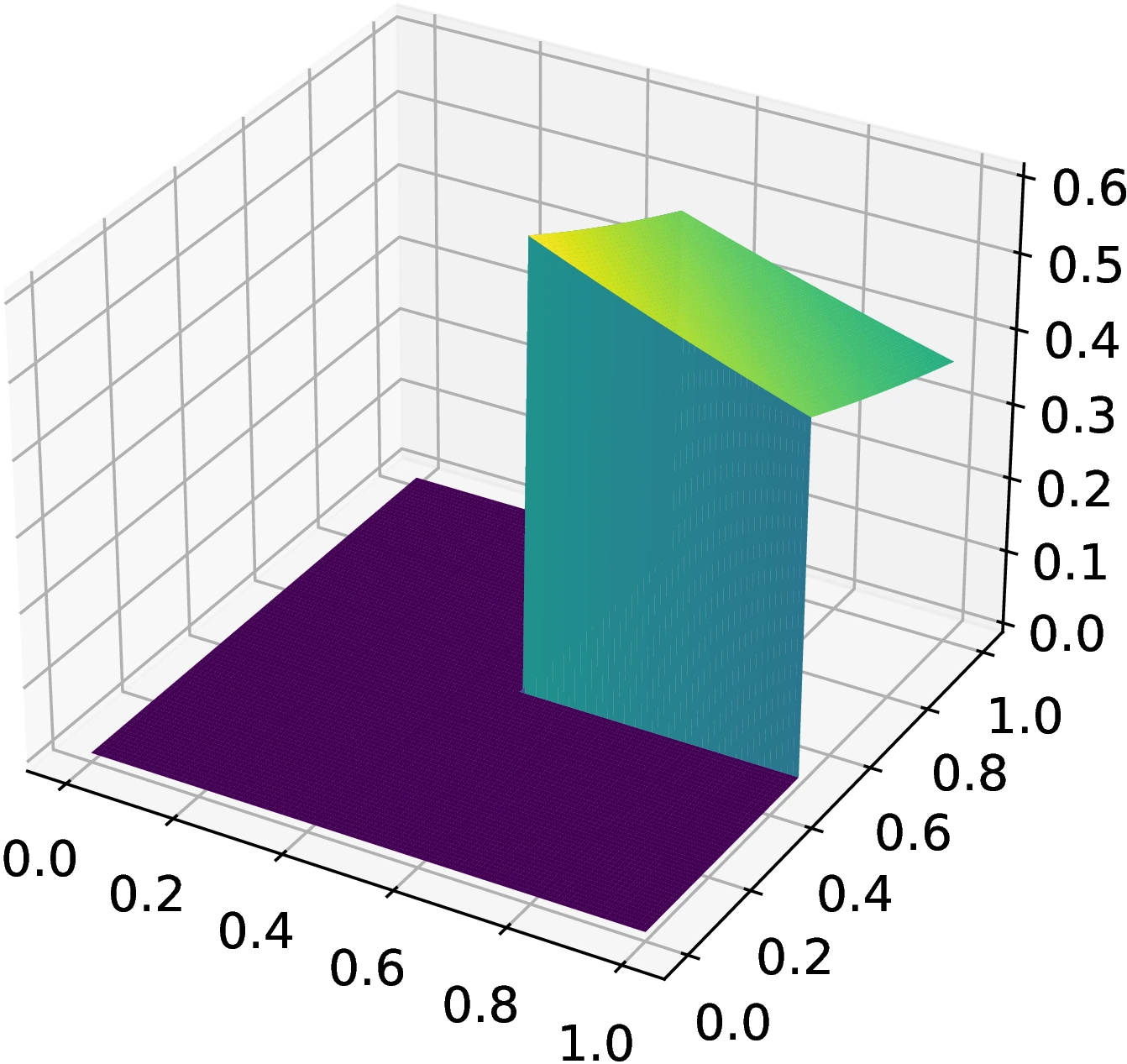
We first examine the function introduced by Genz [18]. This function, visualized in Figure [15]. This functions is of interest due to its discontinuity as this may prove challenging for numerical integration methods; the uniformity properties of the sequences become especially important for this function. Given random parameters (drawn from uniform distribution ) and (), the integrand is given by:
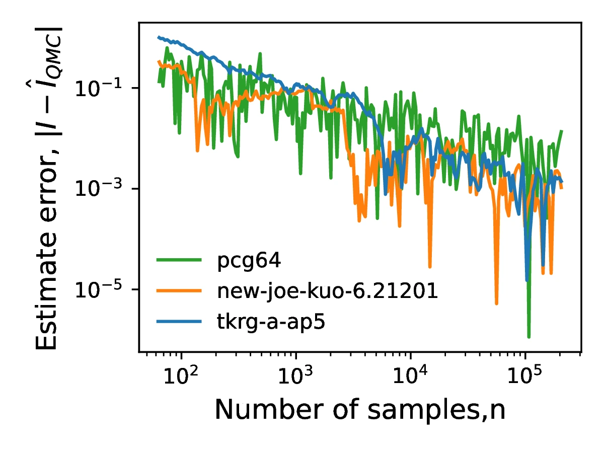
For the purposes of illustration, both and are fixed at 0.5. The expected value of the discontinuous function when is 1.201e-6 (3 d.p.). Figures [15a] and [15b] show the 3D surface projections and absolute numeric error estimates, respectively. There is a steady decrease in the error estimates observed for all three generators. Furthermore, the gradient of tkrg-a-ap5 is the greatest, while that of pcg64 is the lowest. The tkrg-a-ap5 errors are less noisy than the others, indicating that estimates of tkrg-a-ap5 are less sensitive to the discontinuity observed in Figure [15a].
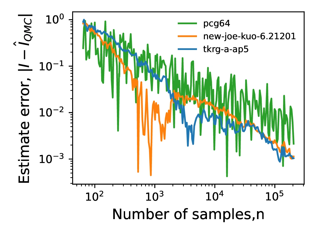
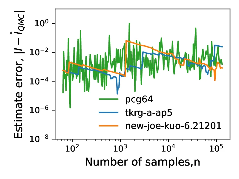
Next, we investigate the integrand provided by Atanassov et al. [5]. Although the function is smooth, as seen in Figure [16]), it cannot be decomposed into sub-integrands:
The expected value of the Atanassov function when is 0.379 (3 d.p.). While the power prevents this function from being decomposed, the smoothness and continuity allow for the successful numerical estimation of the integral (Figure [16a]). These features also allow the LDS generators to effectively compete with the pseudo-random generator.
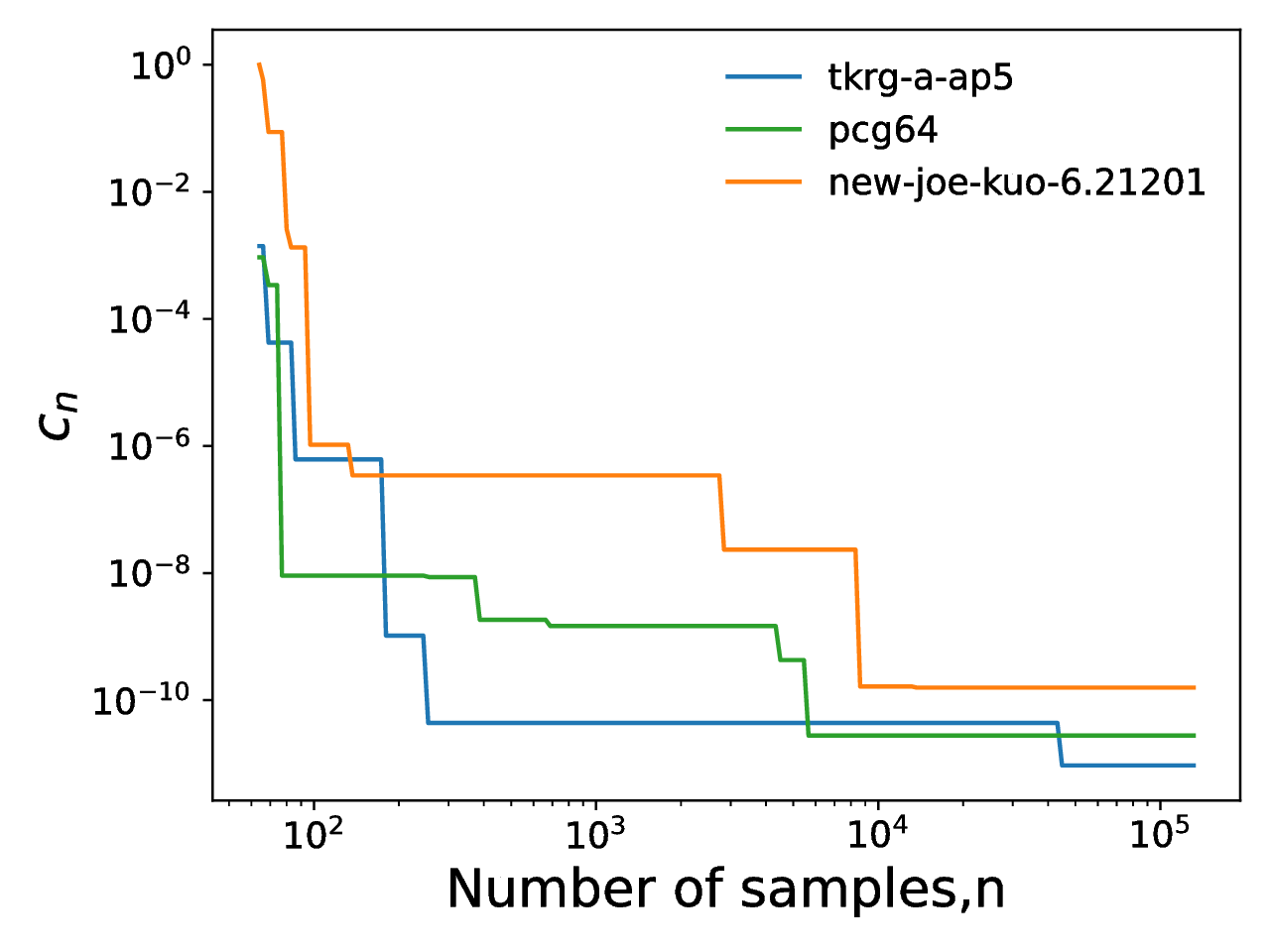
As noted in [16], using low discrepancy sequences allows one to evaluate improper integrals - those which
cannot be computed using conventional quadrature techniques owing to a singularity of the integrand at the origin . As the singularity occurs only at the point , we can obtain successively better approximations to the integrals values by using an increasing amount of points. As this point number increases, they fill the interval with greater uniformity, shrinking the interval around the singularity - represents the position of the closest point from along any of the dimensions. The evolution of with increasing can be used as a measure of uniformity of distribution of the points, defined by:
Here, is the point in the d-dimensional sequence. In effect, is the minimum of any dimensions away from zero. The for different sample sizes are shown in Figure [17] for pcg64, new-joe-kuo-6.21201 and tkrg-a-ap5. It can be seen that larger sample sizes lead to lower values of and thus more uniformly distributed sequences. While pcg64 dominates for sample sizes of less than , tkrg-a-ap5 is the most uniformly distributed for greater sample sizes.
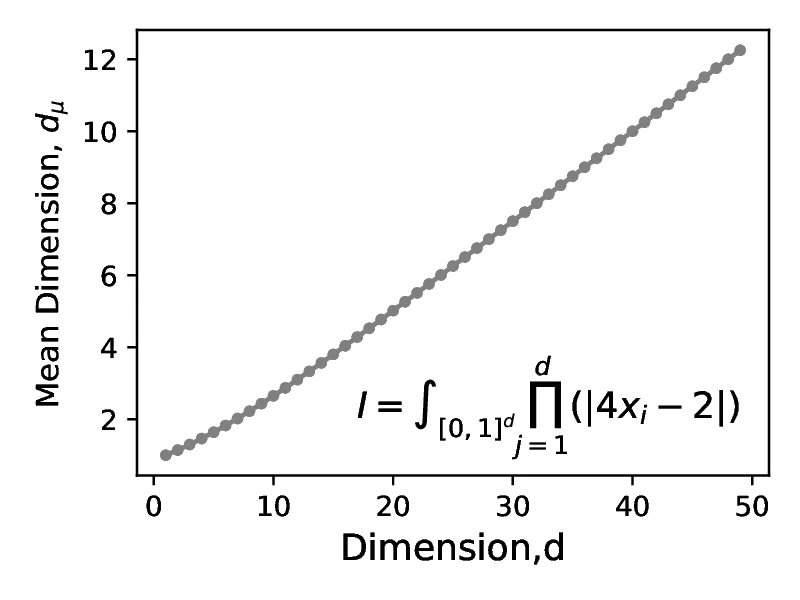
In the following section, we compare the generated sequences on test integrals roos_and_arnold_2, roos_and_arnold_3 and joe_kuo_1 (Section [Classes of test integrals]). These are selected to illustrate the effect of integral properties like effective dimension and discontinuities on convergence of the estimators. All convergence plots are shown for the versions of the integrals. The examples help illustrate that low discrepancy sequences may produce comparable or better results as well as exhibit different convergence properties to pseudo-randon sequences and that this depends not only on the sequences but also on the integral. In the first of these experiments, shown in Figure [18], we consider the roos_and_arnold_2 function:
The function is formed as a product of linear `v` type components for each dimension inducing a highly discontinuous function whose mass concentrates on the edges of the [0,1] domain. The discontinuities of the function concentrate the mass in progressively smaller regions in the domain as dimensionality increases, thus causing large jumps in the estimate when a point `gets lucky` and lands in a high value region, as shown in Figure [18a]. Another feature is that the effective dimension scales linearly with nominal dimension (as shown in Figure [18b]). As a result low discrepancy sequences (QMC) do not produce improved convergence when compared with pseudo-random sequences (MC). The second experiment uses the roos_and_arnold_3 (Figure [19]) function:
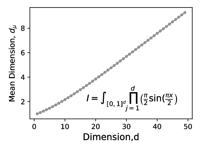
Contrary to roos_and_arnold_2 this function concentrates its mass around the midpoint of the unit interval (=0.5) and does not contain sharp discontinuities. Consequently we see a smoother variation and a gradual reduction in estimator error. Similarly to the previous case the effective dimension also grows linearly with increasing nominal dimension but with a lower gradient (0.18 for roos_and_arnold_3 compared with 0.22 for roos_and_arnold_2). This linear increase in effective dimension can again be a potential justification for similar performance of the estimator with using QMC and MC. It should however be noted that for certain numbers of samples, the QMC estimate error is orders of magnitude smaller than the MC estimate, potentially explained by the sequence being `balanced` at that sample count (). Finally, joe_kuo_1 represents a similar function roos_and_arnold_3 but adds a weighting to each dimensions contribution to the integrals value by means of the present in both numerator and denominator:

This decay in the contribution of higher dimensions causes the effective dimension of the integral to be low, reaching only 1.7, compared to the nominal dimension () of the integral, as shown in Figure [20]. While the effective dimension is low, the estimate convergence rate of QMC does not appear to improve over MC for the considered range of , unlike joe_kuo_2 shown in Figure [13]). This may be attributed to the functional form of the components of this integral, again being concentrated around the edge of the [0,1] integration domain. Consequently the improved convergence of QMC relative to MC in this case likely manifests only at a number of samples, greater than . This underlines the importance of considering all available information about the integral, not only the effective dimension when using QMC.