Probabilistic graphical model for student loan repayments

This report presents a probabilistic graphical model for analyzing and predicting student loan repayments, leveraging the Stochastic Earnings Path (StEP) model previously employed by the UK’s Department for Business, Innovation & Skills (BIS). The StEP model integrates stochastic elements into earnings projections to provide a nuanced understanding of repayment behaviors under varying economic conditions. By coupling the StEP model with a probabilistic graphical model, this approach aims not only to improve the accuracy and interpretability of student loan repayment forecasts but also to provide a framework for scenario analysis and what-if analysis.

Student loan repayment forecasting plays a critical role in public policy and financial planning. The BIS employed the StEP model to model future graduate earnings and associated repayment patterns. This report builds on that foundation, introducing a probabilistic graphical model that enhances predictive capabilities while maintaining transparency and adaptability.

The proposed approach aims to:

• Integrate stochastic earnings modeling with a graphical representation to capture the dependencies among key variables.
• Provide policymakers with tools for scenario analysis under varying economic assumptions.
• Enhance the accuracy of long-term student loan repayment projections.
• Enable analysis of full distributions on output results and key metrics.

The Stochastic Earnings Path (StEP) model, specifically its third iteration (StEP3), forecasts the cost of student loans within an income-contingent repayment system. It combines historical data, macroeconomic projections, and borrower characteristics to estimate repayment behaviors and the Resource Accounting and Budgeting (RAB) charge—the portion of the loan value not expected to be repaid.

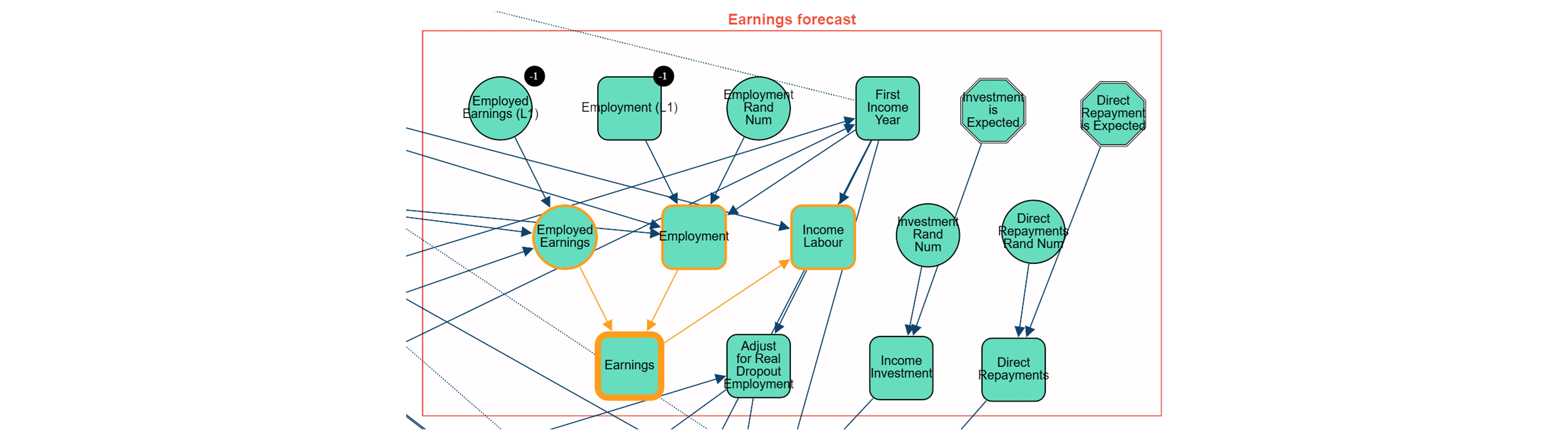
Earnings Forecasting: Individual earnings paths are predicted using regression models that factor in historical data, borrower characteristics, career progression, age, gender, course subject, and institution.

Macroeconomic Inputs: Economic forecasts from the Office for Budget Responsibility (OBR), including earnings growth, inflation rates, and discount rates, are incorporated. Real earnings and repayment estimates are adjusted for inflation (RPI+2.2%).

Loan Repayment Parameters: These include repayment thresholds, interest rates, maximum repayment periods, obligatory and voluntary repayments, and overseas payments.

Borrower Characteristics: The model considers non-employment likelihoods, mortality, disability, and migration patterns, drawing on data from the International Passenger Survey (IPS).

Data Sources: Key datasets include Student Loans Company (SLC) administrative data, British Household Panel Survey (BHPS), Labor Force Survey (LFS), and others for demographic and loan take-up insights.

The primary outputs include:

• The RAB charge, expressed as a percentage of the loan value not expected to be repaid in Net Present Value (NPV) terms.
• Earnings paths and repayment projections across borrower cohorts.

Probabilistic graphical models (PGMs) are frameworks for representing and reasoning about complex systems using probability theory. They consist of a graph-based structure where nodes represent random variables and edges denote probabilistic dependencies. PGMs provide a structured way to handle uncertainty and dependencies in real-world problems, making them essential in various domains from healthcare to finance.

Bayesian networks, a subset of probabilistic graphical models, are directed acyclic graphs (DAGs) that encode conditional dependencies between variables. These networks enable:

Representation of Uncertainty: Probabilities associated with different outcomes based on evidence.

Inference: Calculation of posterior probabilities given observed data, useful for understanding repayment likelihoods under various economic conditions.

Scenario Testing: Simulation of different policy changes and their effects on repayment probabilities. For instance, in the context of student loans, a Bayesian network can model how changes in interest rates or economic growth impact the probability of repayment success.

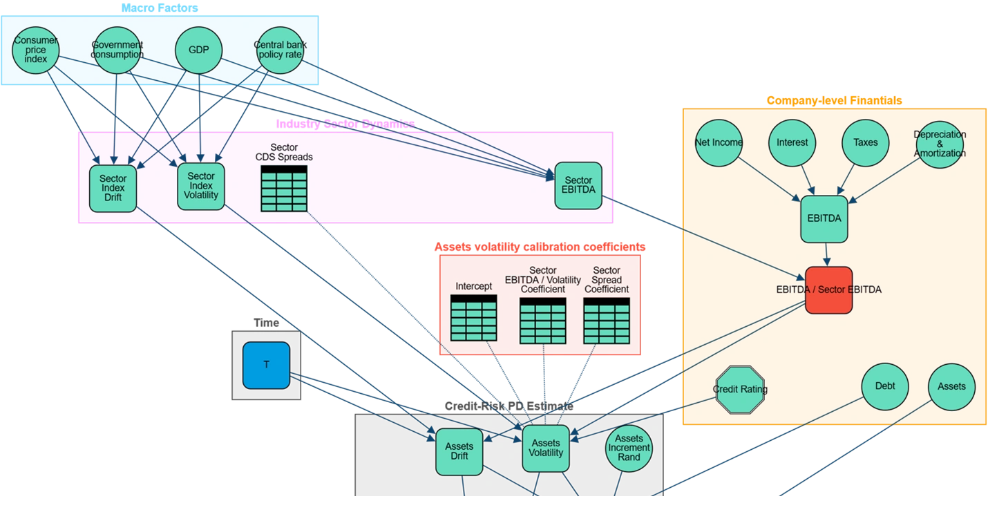
The student loan repayment PGM is structured as follows:

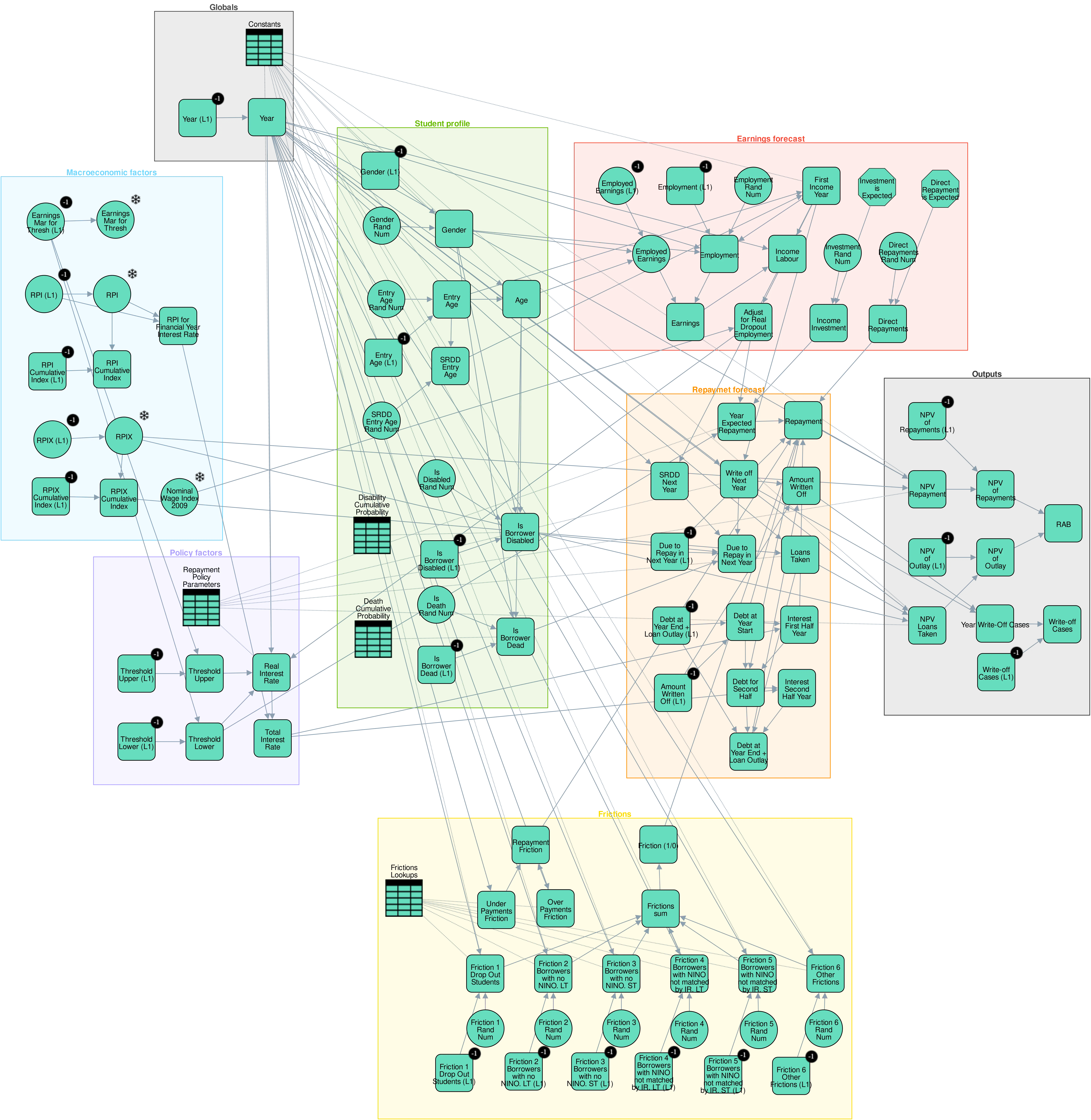
Globals: Variables that universally affect all domains, such as year and macroeconomic and policy factors constants.

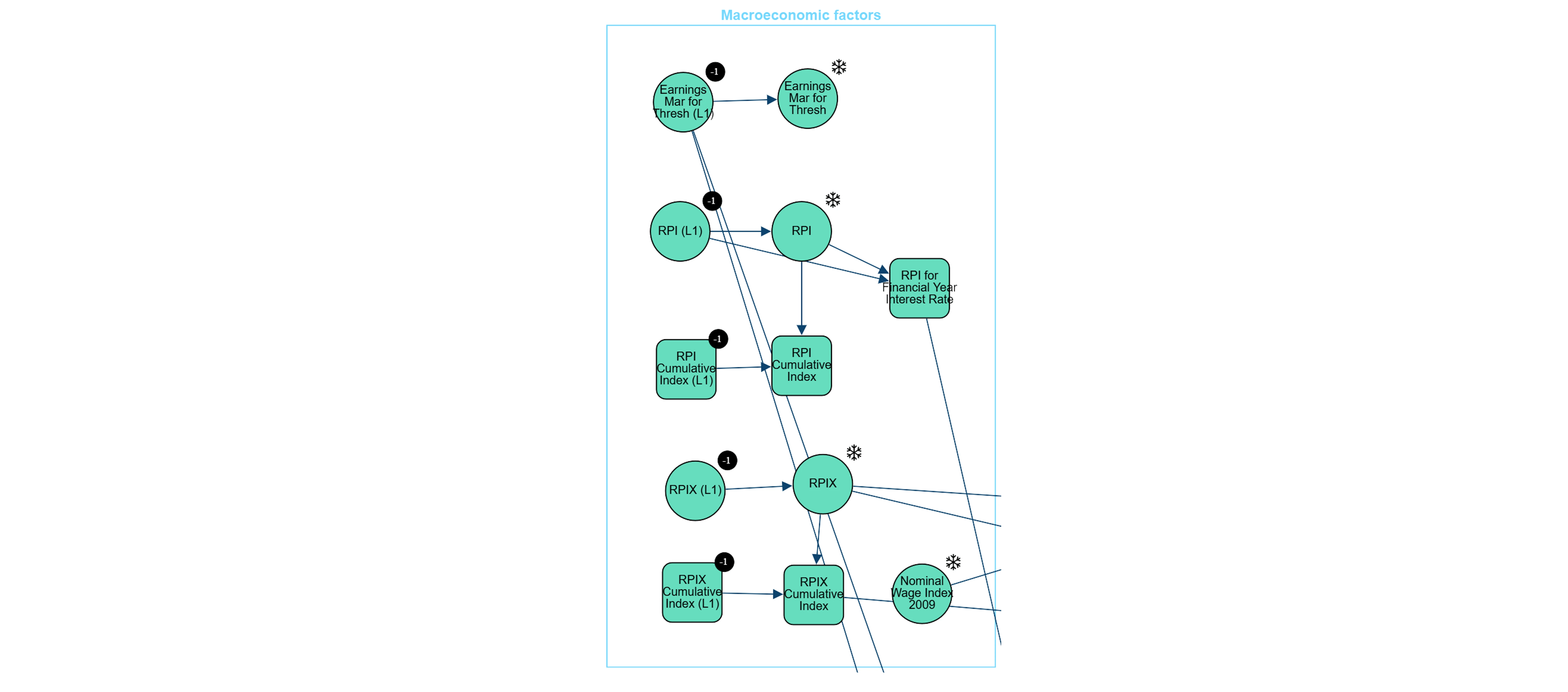
Macroeconomic Factors: Includes variables that tracks inflation and earnings projections like rental prince index (RPI), earnings and nominal wage index.

Policy Factors: Government and institutional policies affecting repayment terms, thresholds, and interest rates.

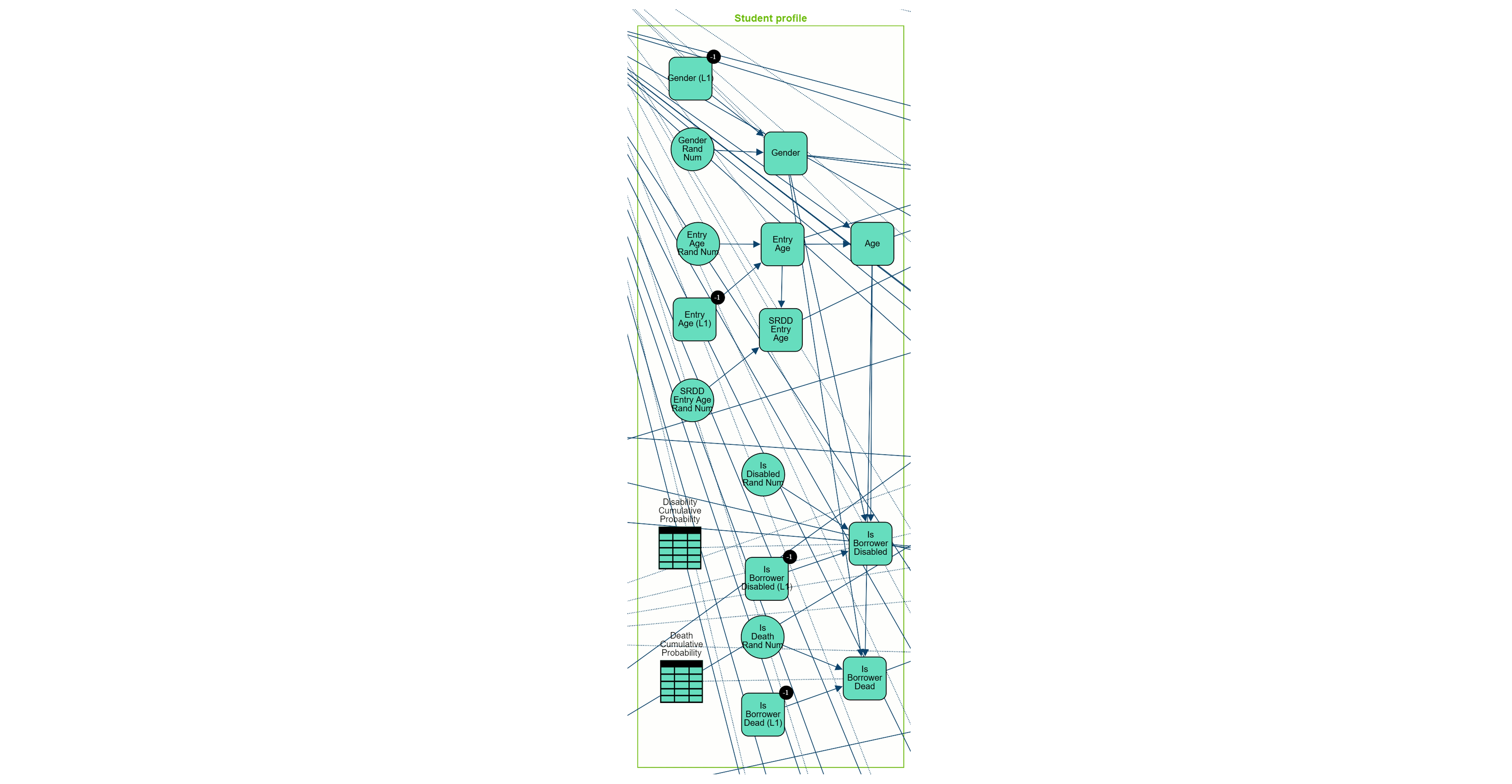
Student Profile: Captures demographic attributes, including age, gender, parental income, graduate income decile, and repayment status.

Earnings Forecast: Focuses on income predictions, employment status, and variations by demographics to estimate repayment capacity.

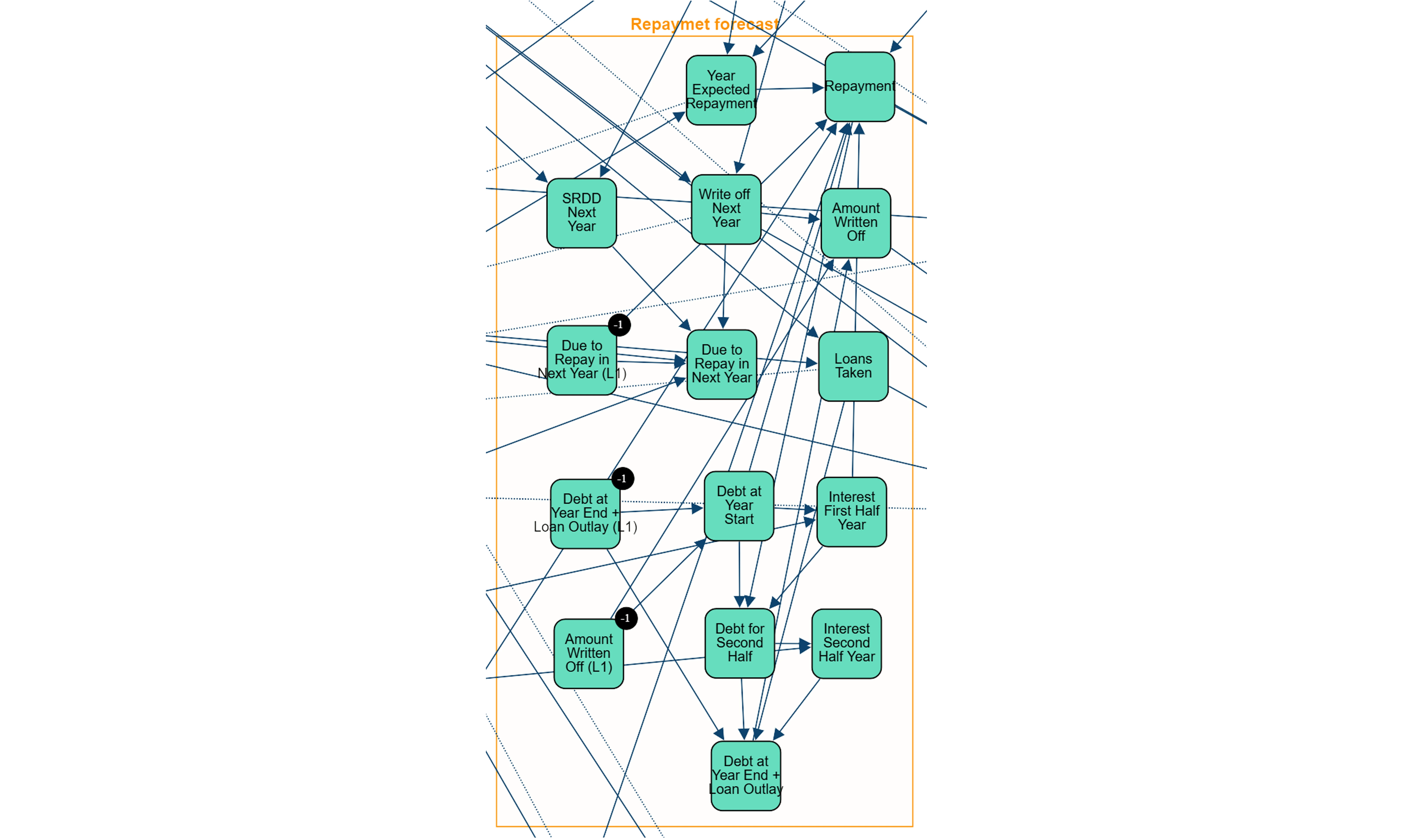
Repayment Forecast: Tracks repayment behaviors, including balances, due amounts, and written-off debts, showing repayment evolution over time.

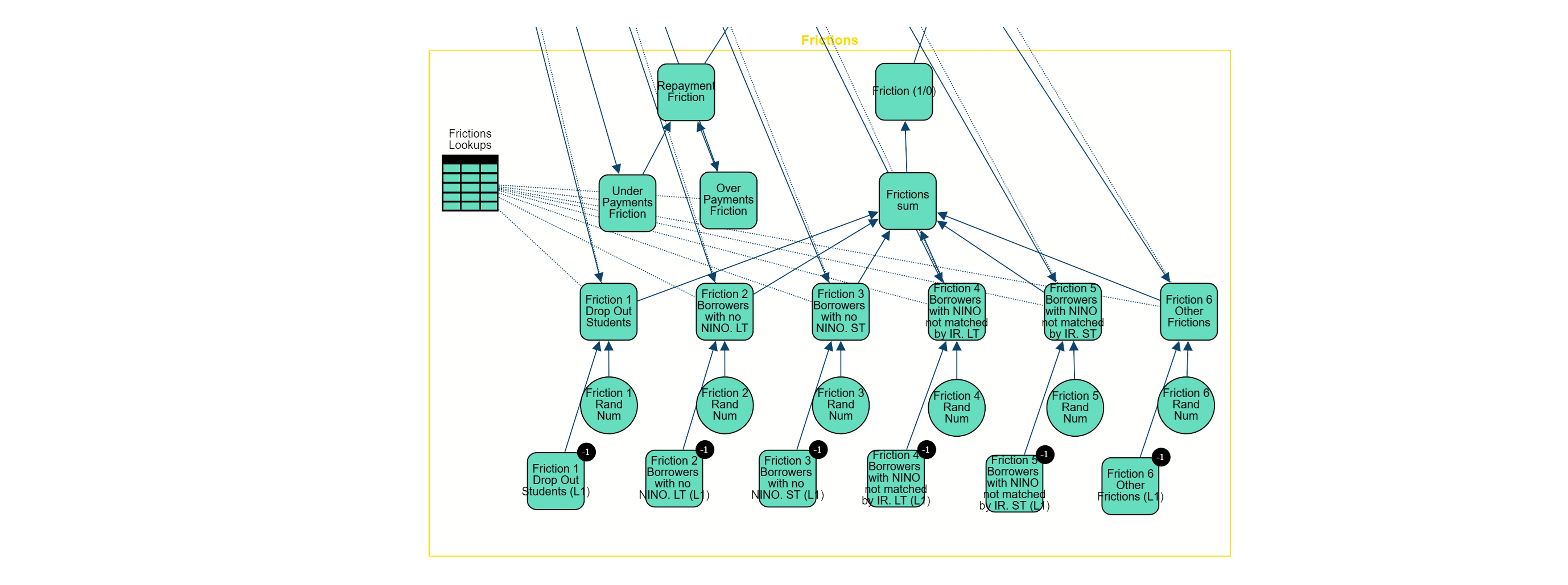
Frictions: Models obstacles like dropouts and administrative issues that affect repayment.

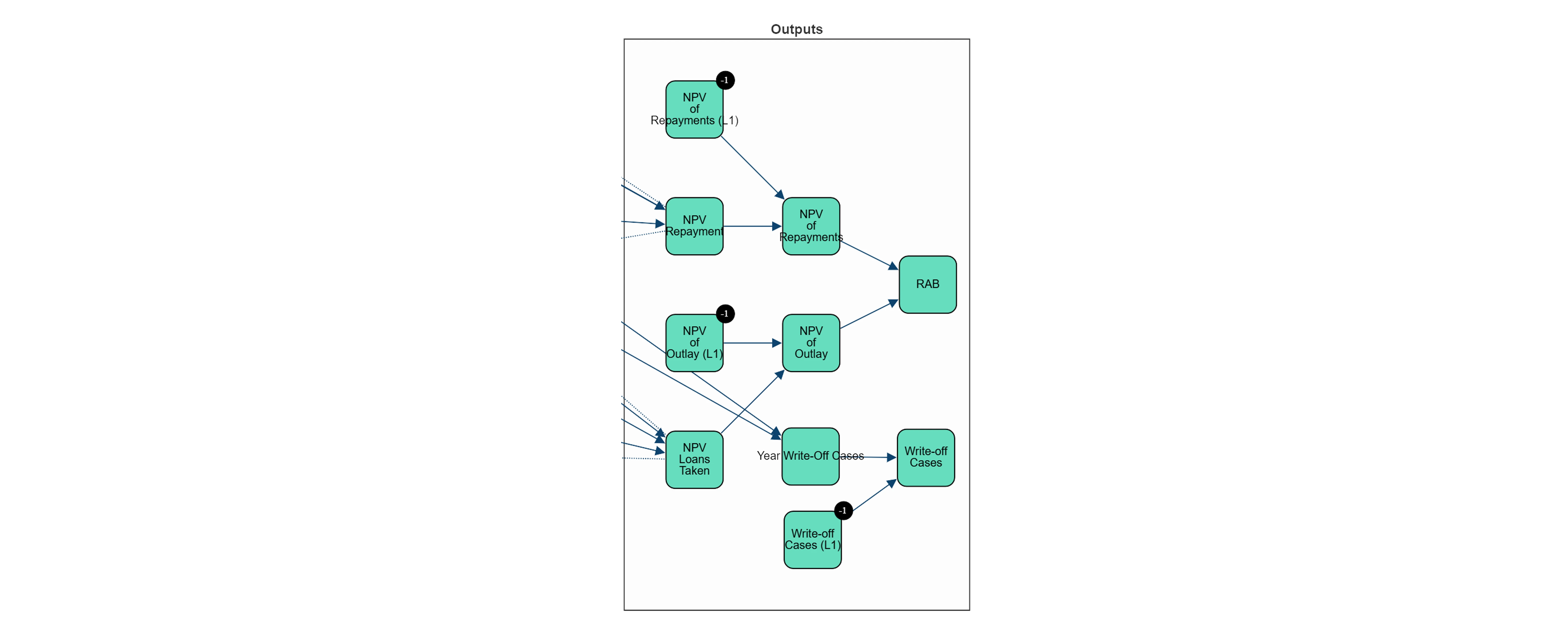
Outputs: Calculates final outcomes, including the NPV of repayments and the RAB charge.

To incorporate time evolution, the proposed network structure is replicated in each time-step. Auxiliary or lagged nodes are included at each step to store values from previous time-steps, facilitating a temporal dependency structure and allowing the model to capture dynamic changes in variables over time.

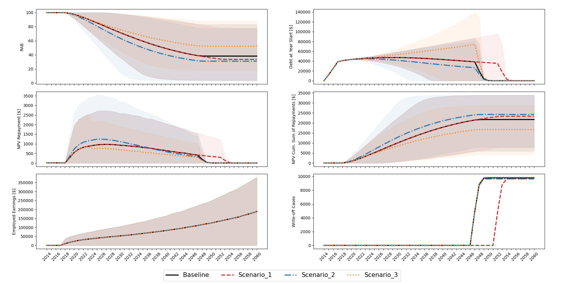
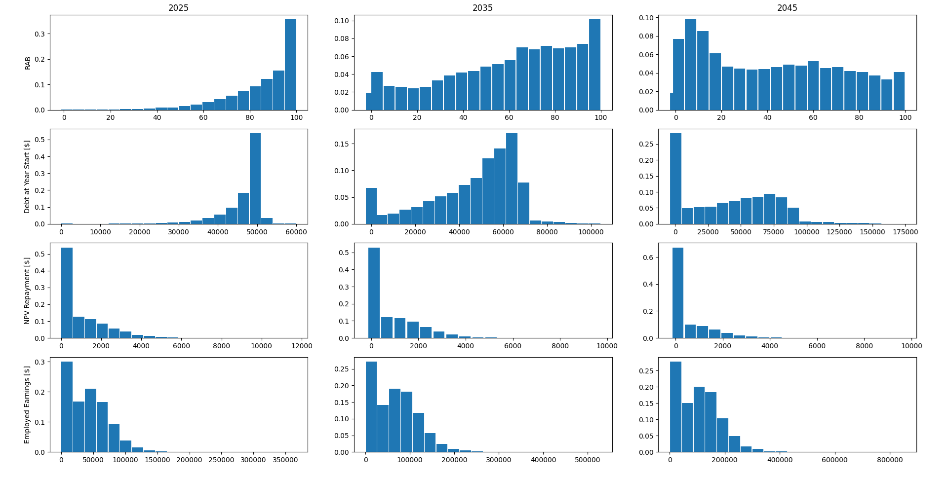
Figures 10 and 11 provide visual insights into the dynamic behavior and distribution of variables modeled by the student loan repayments PGM. Figure 10 presents the time evolution of six critical variables under three different policy scenarios. In Scenario 1, the maximum repayment term increases from 30 to 35 years, Scenario 2 assumes an increase in the repayment rate from 9% to 12% and Scenario 3 considers a higher inflation scenario, with the RPI index increasing from 3% to 5%.. Figure 11, on the other hand, shows the distribution of variables at three specific time points—2025, 2035, and 2045. The rows represent different variables, and the columns correspond to the selected years, providing a snapshot of how these variables shift over time under the model’s projections. Together, these figures highlight both temporal trends and cross-sectional variability, offering policymakers robust tools for understanding and forecasting loan repayment dynamics.

By integrating the StEP model with a probabilistic graphical framework, this approach provides a robust, flexible tool for modeling student loan repayments. The enhanced predictive accuracy and policy simulation capabilities address key challenges in student loan portfolio management, supporting informed decision-making in education financing.