Probabilistic Graphical Model for Credit Risk

Adrien Papaioannou

Andres Oliva Denis

December 9, 2024

ABSTRACT

This report presents an enhanced structural credit risk model built on the classical Merton framework, extended via a Bayesian network to capture dependencies across macroeconomic forecasts, sector dynamics, and firm-specific financial metrics. We calibrate using historical CDS spreads and demonstrate how this approach refines probability of default (PD) and expected loss (EL) estimates.

1. Introduction

Credit risk assessment is central to financial risk management and regulatory compliance. In the traditional Merton model, a firm's equity is viewed as a European call option on its assets, with default when asset value falls below a threshold at debt maturity. However, real-world complexities—interactions among economic cycles, sector performance, and firm financial health—motivate a probabilistic graphical extension. Our Bayesian network integrates continuous macro forecasts (CPI, GDP, policy rates), sector-level dynamics, and firm-level metrics (EBITDA, leverage, credit rating) into a unified framework, allowing joint inference and scenario analysis.

2. Methodology

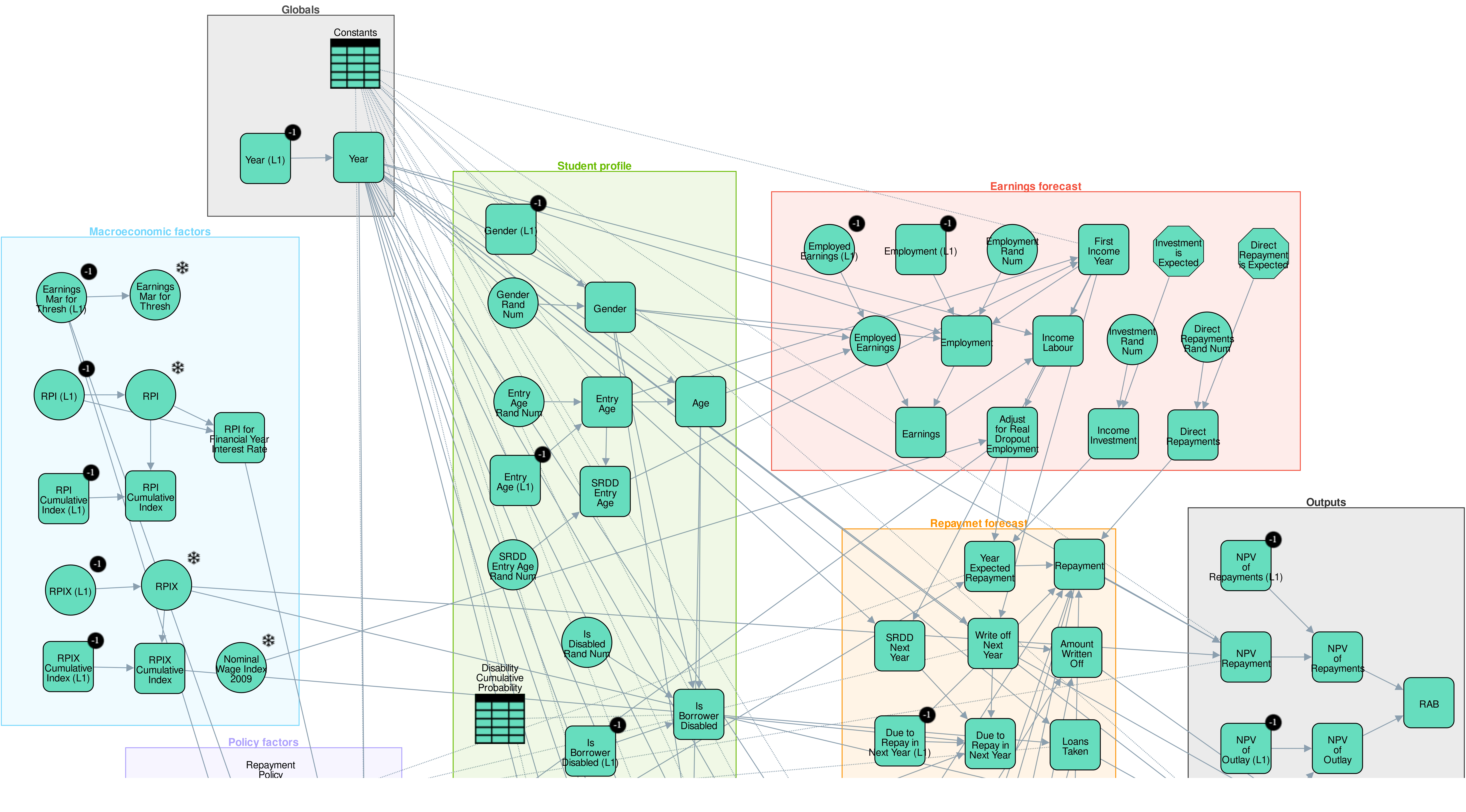
We specify a directed acyclic graph with interlinked layers:

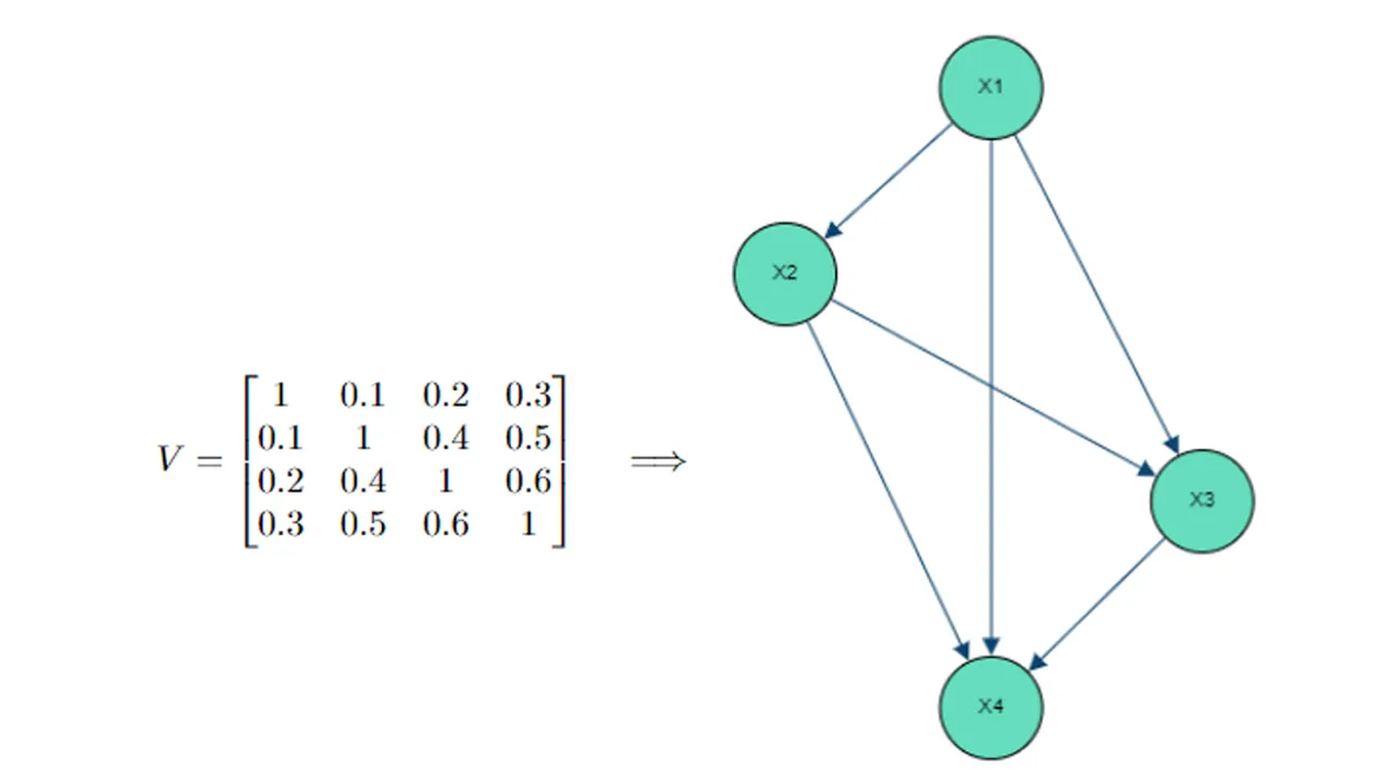
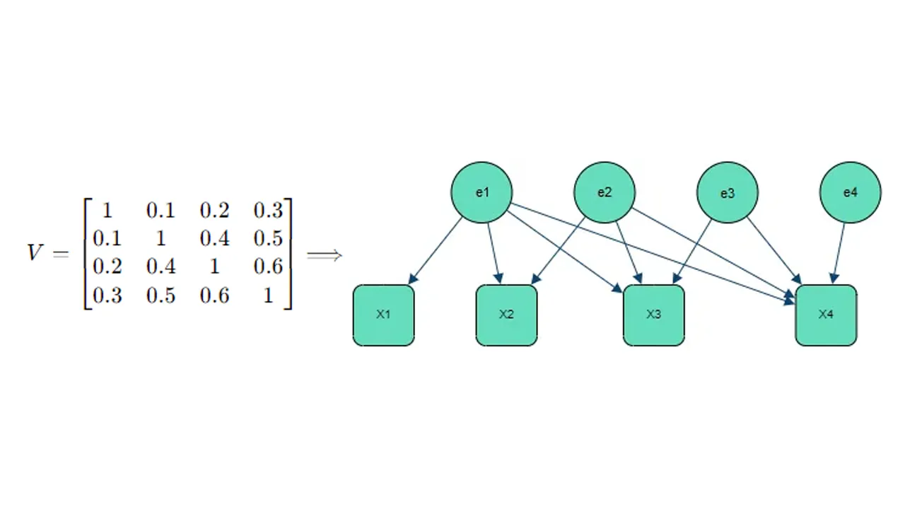
Macroeconomic Factors (MF): Joint forecasts of CPI inflation, GDP growth, government spending, and central bank policy rate, modeled as a multivariate normal distribution.

Sector Dynamics (SD): Sector drift and volatility captured by linear regressions on MF, plus white-noise residuals.

Firm Properties (FP): Observed at time: EBITDA, total assets, total debt, credit rating, and normalized EBITDA-to-sector ratio.

Asset Process & Default Module: Firm asset value evolves log-normally:

$d \ln A_t = \left( \mu_{\text{sector}} + \alpha_i \right) dt + \left( \sigma_{\text{sector}} + \beta_i \right) dW_t$

with $a_i$ and $ß_i$ firm-specific drift and volatility adjustments. Probability of Default at maturity is

$PD = 1 - N\left( \frac{\ln A_t - \ln L}{\sigma_A \sqrt{T}} \right)$

Expected Loss (EL): $EL=PD·LGD·EAD$ , where loss given default (LGD) and exposure at default (EAD) are calibrated to long-run sectoral averages.

3. Structural Credit Risk PGM

The structural credit risk PGM is structured as follows:

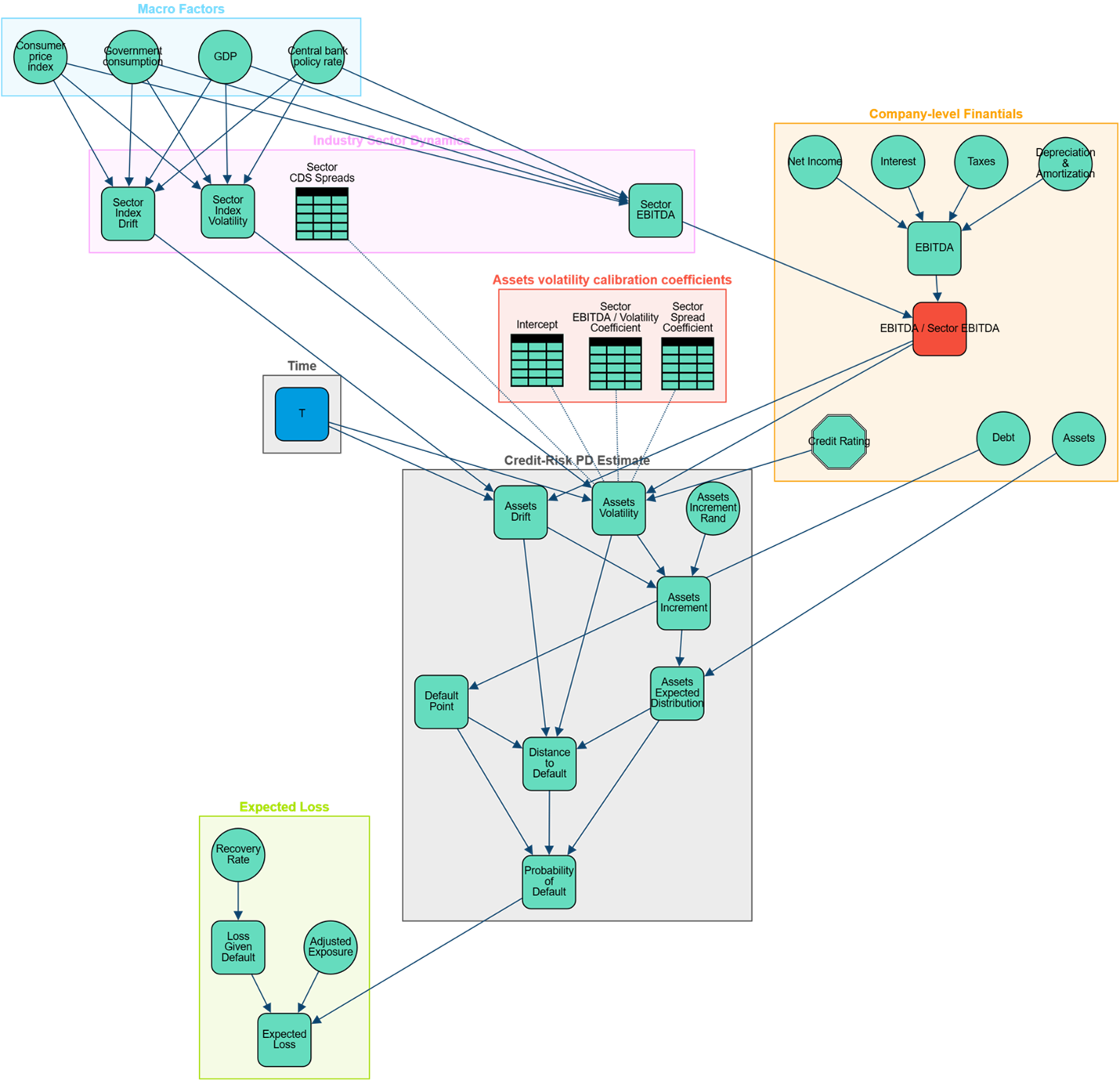
Figure 1. Bayesian network of the structural credit risk model

Macro Factors: Macroeconomic variables are modeled as continuous random variables that follows a normal distribution that describes forecast and its uncertainty.

Figure 2. PGM nodes within ‘Macro Factors’ group.

Industry Sector Dynamics: Sector index drift, volatility and EBITDA are modeled as linear combination of the macroeconomic factors forecast.

Figure 3. PGM nodes within ’Industry Sector Dynamics’ group.

Company-level financials: Company-level current financials. These include net incomet, testeres, taxes, debt, assets, credit rating, EBITDA and EBITDA/sector EBITDA ratio.

Figure 4: PGM nodes within ‘Company-level Financials’ group.

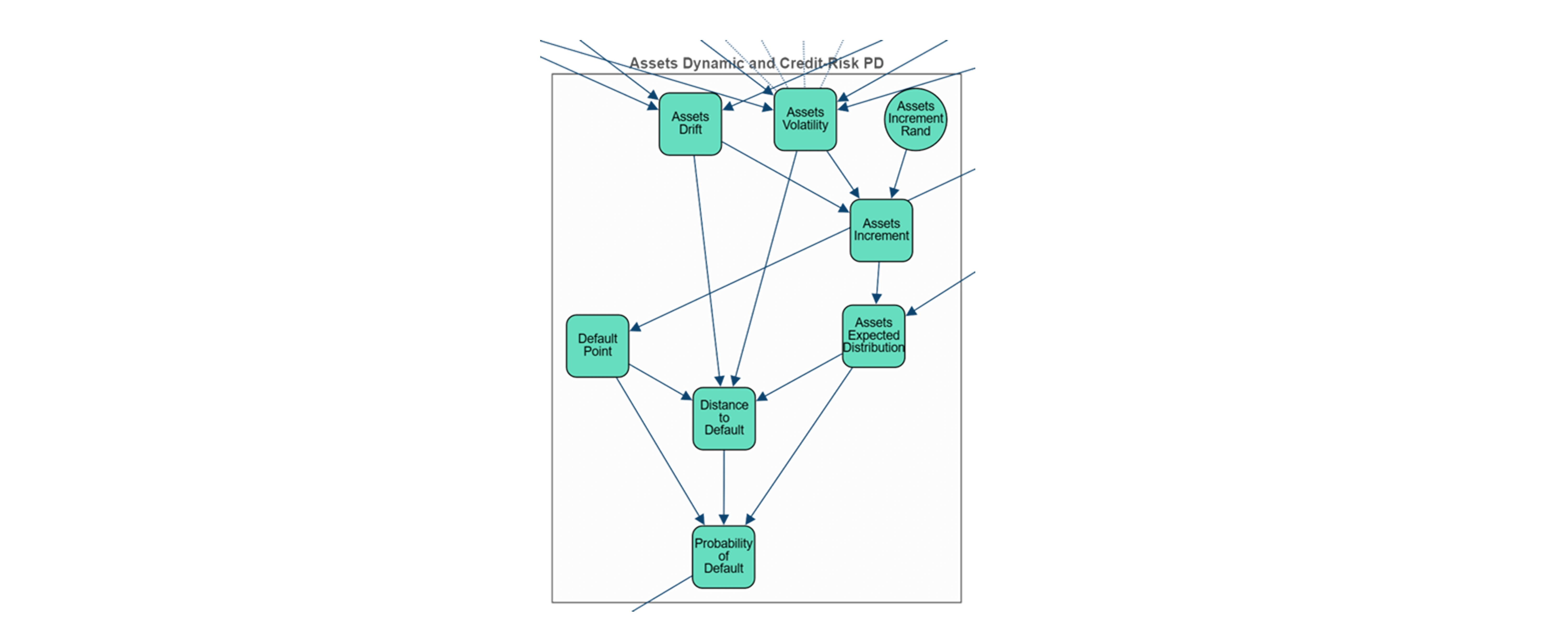
Assets Dynamic and Credit-Risk PD: Asset log-normal expected distribution and probability of default computation.

Figure 5: PGM nodes within ‘Assets Dynamic and Credit-Risk PD’ group.

Expected loss: expected financial loss.

Figure 6: PGM nodes within ‘Expected Loss’ group.

4. Results

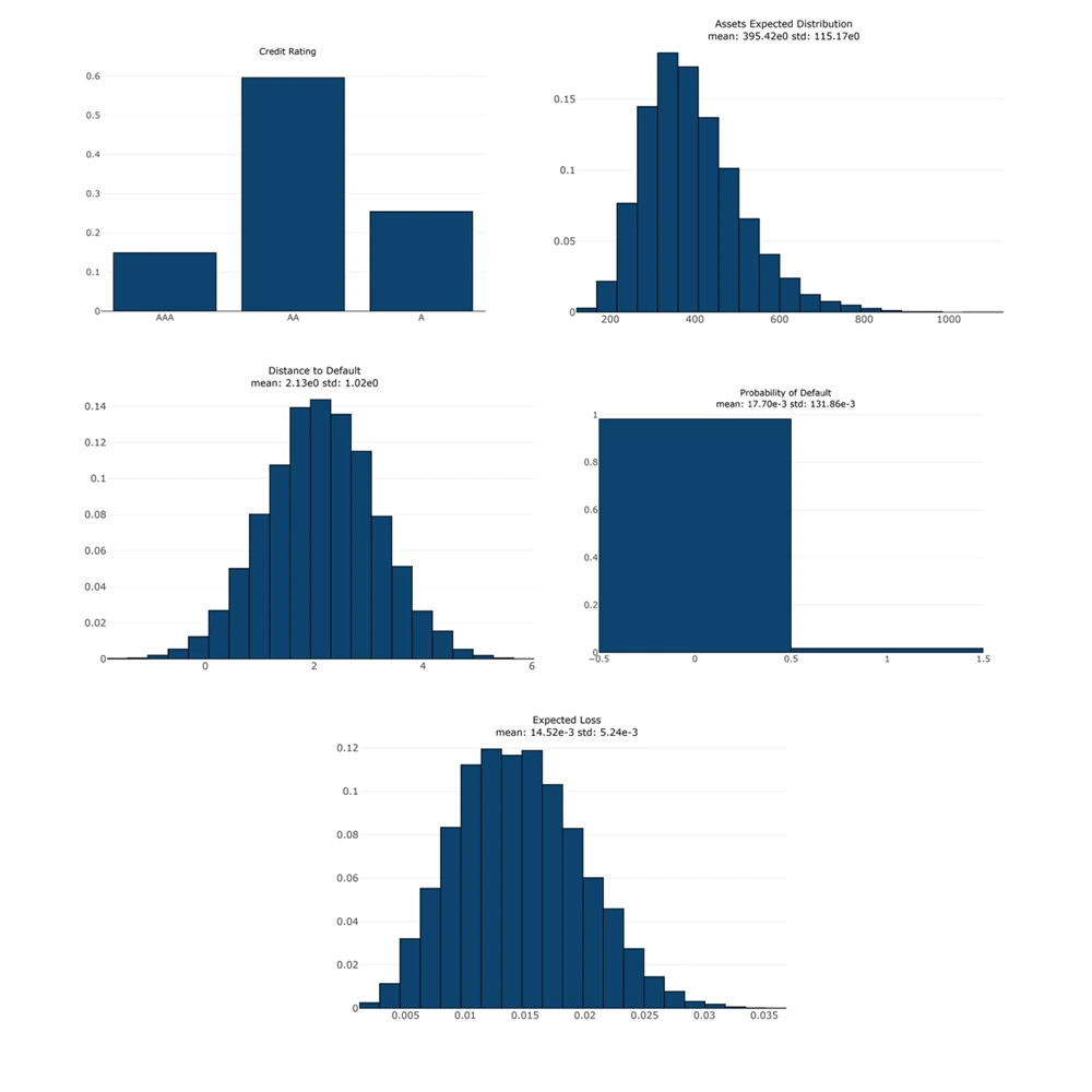
We leverage Monte Carlo sampling (10,000 paths) to generate empirical distributions. Figure 6 below illustrate these sampled distributions for our representative industrial firm (Shell) and five key risk metrics: firm asset values at horizon, distance to default (DD), probability of default (PD), and expected loss (EL).

Figure 7. Variables distributions output from model. a) Credit Rating. b) Assets Expected Distribution. c) Distance to Default. d) Probability of default. e) Expected loss

5. Conclusion

This Bayesian-network-enhanced structural model refines traditional Merton-based credit risk estimates by explicitly modeling dependencies between macroeconomic conditions, sector dynamics, and firm-specific characteristics. The modular Bayesian framework also affords straightforward extensions: multi-firm contagion modeling, time-varying sector correlations, and real-time Bayesian updating with market data. Overall, this approach provides risk managers and regulators with a robust, flexible toolset for quantifying credit risk under uncertainty.

References

Merton, R. C. (1974). On the Pricing of Corporate Debt: The Risk Structure of Interest Rates. Journal of Finance, 29(2), 449–470.

Black, F., & Scholes, M. (1973). The Pricing of Options and Corporate Liabilities. Journal of Political Economy, 81(3), 637–654.

Daphne Koller and Nir Friedman. Probabilistic graphical models: principles and techniques. MIT press, 2009.