Plume Migration - II
In this section, we review how we can model the average saturation behind the front of CO2. In instances where the relationship between input and output is too complex or simply does not exist, we can use calibration methods to 'tune' a model. TKRISK continuous nodes allow such approach. In the example of the average saturation in the plume, the theory of hyperbolic systems of conservation laws governs the displacement mechanism and hence the property of interest. We have a complex non-linear relationship between rock/fluid properties and the fractional flow tangent that will give the average saturation of CO2 that will itself drive the speed of expansion of the plume... We can use an existing model to build a multi-linear model of the average saturation using ordinary least square regression. This leads to a graph where the CO2 front speed propagation can be tied to the reservoir properties.
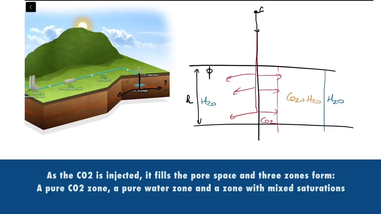
The missing component is the computation of the average saturation behind the front.
For this we need to refer to the fractional flow (fw) which depends on the mobility ratio of the two phases M defined by the ratio of their respective viscosities and relative permeabilities
These later characterize the “ease to flow” of a given phase
These relationships are developed in the Buckley and Leverett Theory (1948) originally created for oil and gas fields but perfectly applicable to CO2 sequestration
The average saturation behind the front is defined by the intersection of the tangent to the fractional flow curve with the unity horizontal
This is obviously a complex calculation that cannot be directly encoded in the graph. This is why we will use a regression model to define the relationship between the average saturation and the mobility components
Back to TKRISK, we can now build the model backwards as before adding more priors as we try to understand the root uncertaintiesWhen we have an explicit relationship (like pressure vs depth), deterministic nodes help us to easily write that relationship. When the explicit relationship cannot be found (like viscosity vs pressure and temperature), we calibrate based on data.
We simulate and get a distribution for the front centered at 25 m from injectors after 10 days of injecting 1000 tons per day of CO2.
After 100 days, the front has travelled further and the distribution centers at 75 m
The following animation shows how the distribution evolves with time as we sample the graph for different times. We also see that the uncertainty grows with time as the spread of the distribution gets wider.
The missing component is the computation of the average saturation behind the front.
For this we need to refer to the fractional flow (fw) which depends on the mobility ratio of the two phases M defined by the ratio of their respective viscosities and relative permeabilities
These later characterize the “ease to flow” of a given phase
These relationships are developed in the Buckley and Leverett Theory (1948) originally created for oil and gas fields but perfectly applicable to CO2 sequestration
The average saturation behind the front is defined by the intersection of the tangent to the fractional flow curve with the unity horizontal
This is obviously a complex calculation that cannot be directly encoded in the graph. This is why we will use a regression model to define the relationship between the average saturation and the mobility components
Back to TKRISK, we can now build the model backwards as before adding more priors as we try to understand the root uncertainties
We simulate and get a distribution for the front centered at 25 m from injectors after 10 days of injecting 1000 tons per day of CO2.
After 100 days, the front has travelled further and the distribution centers at 75 m
The following animation shows how the distribution evolves with time as we sample the graph for different times. We also see that the uncertainty grows with time as the spread of the distribution gets wider.
Up Next: