Plume Migration - I
We quantify the evolution of the CO2 plume during the injection process. We use TKRISK to model the displacement of original fluids (brine, hydrocarbon) in the geological formation with injected CO2. We are able to quickly build a simple radial flow model of the injection process and propagate key uncertainties (average porosity, injection rate as an example) to model the radius of the CO2 plume as a function of time. This example shows how one can build a graph based model of a transient variable using time as a deterministic input.
We continue our journey trying to understand how far the CO2 injected travels in the subsurface
We model the injection string going through a reservoir with thickness h, porosity \phi that is originally filled with Water. As the CO2 is injected, it fills the pore space and three zones form: A pure CO2 zone, a pure water zone and a zone with mixed saturations
The saturation of CO2 decreases as we depart from the injector following a trend similar to the one displayed in the graph with the apparition of a front at a distance r_f
We want to know how fast this front moves as it informs us on how far the CO2 moved away from the well
The relationship between injection rate and radius of the plume is determined by a radial flow equation (dr/dt=…)
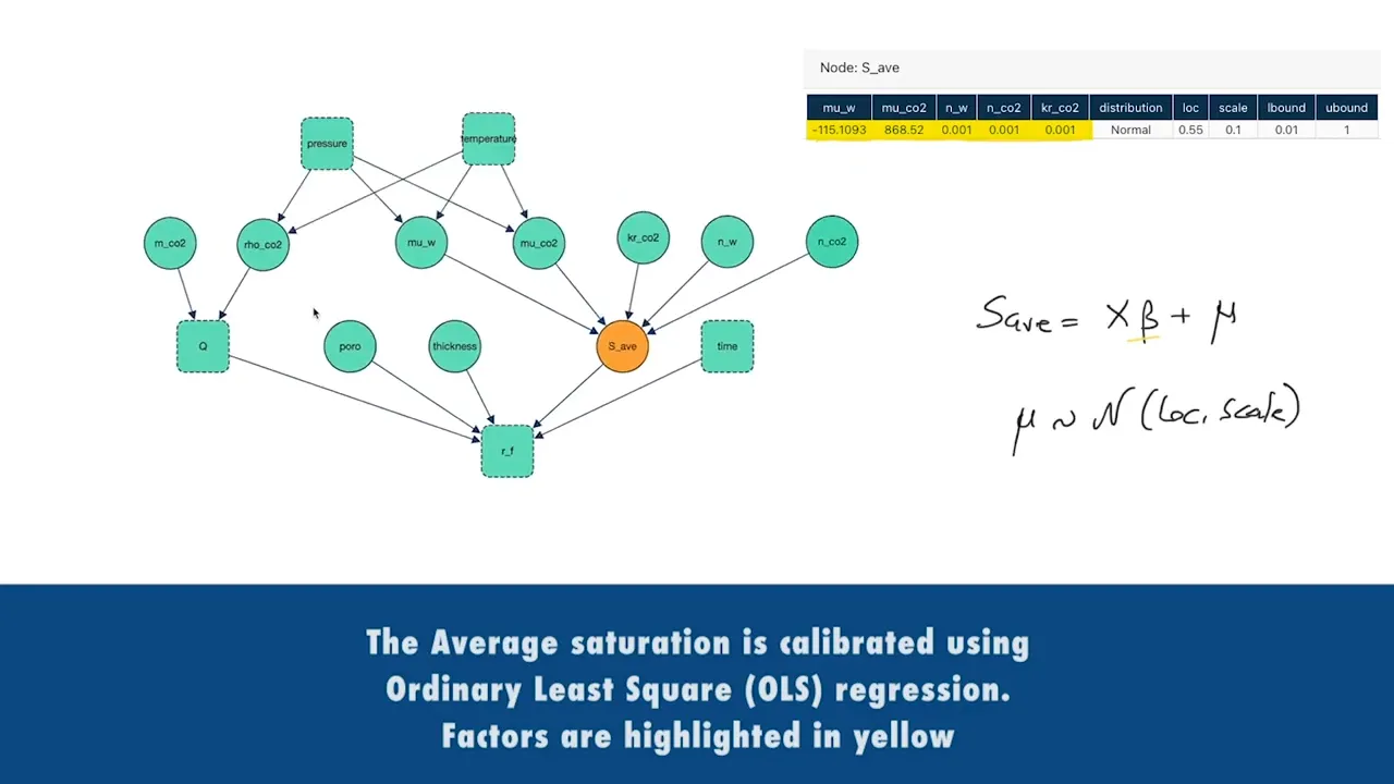
The key unknown in this equation is the average saturation behind the front which characterizes how much water is displaced by the CO2
The integration by part of this differential equation allows us to establish a relationship between the front radius and the total amount of CO2 injected
We display the various units in this relationship
In TKRISK, we can specify the units and description of variables to ensure consistency. The relationship can easily be modeled using a series of continuous and deterministic nodes. We notice the “time” variable modeled as a deterministic node.
We encode the expression derived in a child deterministic node run a first simulation
We continue our journey trying to understand how far the CO2 injected travels in the subsurface
We model the injection string going through a reservoir with thickness h, porosity \phi that is originally filled with Water. As the CO2 is injected, it fills the pore space and three zones form: A pure CO2 zone, a pure water zone and a zone with mixed saturations
The saturation of CO2 decreases as we depart from the injector following a trend similar to the one displayed in the graph with the apparition of a front at a distance r_f
We want to know how fast this front moves as it informs us on how far the CO2 moved away from the well
The relationship between injection rate and radius of the plume is determined by a radial flow equation (dr/dt=…)
The key unknown in this equation is the average saturation behind the front which characterizes how much water is displaced by the CO2
The integration by part of this differential equation allows us to establish a relationship between the front radius and the total amount of CO2 injected
We display the various units in this relationship
In TKRISK, we can specify the units and description of variables to ensure consistency. The relationship can easily be modeled using a series of continuous and deterministic nodes. We notice the “time” variable modeled as a deterministic node.
We encode the expression derived in a child deterministic node run a first simulation
Up Next: